ls4 R Basics
Before we get started with this analysis we are reviewing some basics.
4.1 Packages
Use install.packages to install the dslabs package.
Tryout the following functions: sessionInfo, installed.packages
4.2 Prebuilt functions
Much of what we do in R is called prebuilt functions. Today we are using: ls, rm, library, search, factor, list, exists, str, typeof, class and maybe more.
You can see the code for a function by typing it without the parenthesis:
Try this:
4.3 Help system
In R you can use ? or help to learn more about functions.
You can learn about function using
help("ls")or
?ls4.4 The workspace
Define a variable.
Use ls to see if it’s there. Also take a look at the Environment tab in RStudio.
Use rm to remove the variable you defined.
4.5 Variable name convention
A nice convention to follow is to use meaningful words that describe what is stored, use only lower case, and use underscores as a substitute for spaces.
For more we recommend this guide.
4.6 Data types
The main data types in R are:
One dimensional vectors: numeric, integer, logical, complex, characters.
Factors
Lists: this includes data frames
Arrays: Matrices are the most widely used
Date and time
tibble
S4 objects
Many errors in R come from confusing data types. Let’s learn what these data types are and useful tools to help us.
str stands for structure, gives us information about an object.
typeof gives you the basic data type of the object. It reveals the lower-level, more fundamental type of an object in R’s memory.
class This function returns the class attribute of an object. The class of an object is essentially type_of at a higher, often user-facing level.
library(dslabs)typeof(murders)[1] "list"class(murders)[1] "data.frame"str(murders)'data.frame': 51 obs. of 5 variables:
$ state : chr "Alabama" "Alaska" "Arizona" "Arkansas" ...
$ abb : chr "AL" "AK" "AZ" "AR" ...
$ region : Factor w/ 4 levels "Northeast","South",..: 2 4 4 2 4 4 1 2 2 2 ...
$ population: num 4779736 710231 6392017 2915918 37253956 ...
$ total : num 135 19 232 93 1257 ...4.7 Data frames
Date frames are the most common class used in data analysis. It is like a spreadsheet. Rows represents observations and columns variables. Each variable can be a different data type.
You can add columns like this:
murders$pop_rank <- rank(murders$population)
head(murders)
state abb region population total pop_rank
1 Alabama AL South 4779736 135 29
2 Alaska AK West 710231 19 5
3 Arizona AZ West 6392017 232 36
4 Arkansas AR South 2915918 93 20
5 California CA West 37253956 1257 51
6 Colorado CO West 5029196 65 30You can access columns with the $
murders$population [1] 4779736 710231 6392017 2915918 37253956 5029196 3574097 897934
[9] 601723 19687653 9920000 1360301 1567582 12830632 6483802 3046355
[17] 2853118 4339367 4533372 1328361 5773552 6547629 9883640 5303925
[25] 2967297 5988927 989415 1826341 2700551 1316470 8791894 2059179
[33] 19378102 9535483 672591 11536504 3751351 3831074 12702379 1052567
[41] 4625364 814180 6346105 25145561 2763885 625741 8001024 6724540
[49] 1852994 5686986 563626but also []
murders[1:5,] state abb region population total pop_rank
1 Alabama AL South 4779736 135 29
2 Alaska AK West 710231 19 5
3 Arizona AZ West 6392017 232 36
4 Arkansas AR South 2915918 93 20
5 California CA West 37253956 1257 51murders[1:5, 1:2] state abb
1 Alabama AL
2 Alaska AK
3 Arizona AZ
4 Arkansas AR
5 California CAmurders[1:5, c("state", "abb")] state abb
1 Alabama AL
2 Alaska AK
3 Arizona AZ
4 Arkansas AR
5 California CA4.8 with
The function with let’s us use the column names as objects:
with(murders, length(state))[1] 514.9 Vectors
The columns of data frames are one dimensional (atomic) vectors.
Here is an example:
length(murders$population)[1] 51How to create vectors:
x <- c("b", "s", "t", " ", "2", "6", "0")Sequences are particularly useful:
seq(1, 10) [1] 1 2 3 4 5 6 7 8 9 10seq(1, 9, 2)[1] 1 3 5 7 91:10 [1] 1 2 3 4 5 6 7 8 9 10seq_along(x)[1] 1 2 3 4 5 6 74.10 Factors
One key data type distinction is factors versus characters:
typeof(murders$state)[1] "character"typeof(murders$region)[1] "integer"Factors store levels and then the label of each level. They are very useful for categorical data.
x <- murders$region
levels(x)
[1] "Northeast" "South" "North Central" "West" 4.10.1 Categories based on strata
The function cut is useful for converting numbers into categories
with(murders, cut(population,
                  c(0, 10^6, 10^7, Inf)))
[1] (1e+06,1e+07] (0,1e+06] (1e+06,1e+07] (1e+06,1e+07] (1e+07,Inf]
[6] (1e+06,1e+07] (1e+06,1e+07] (0,1e+06] (0,1e+06] (1e+07,Inf]
[11] (1e+06,1e+07] (1e+06,1e+07] (1e+06,1e+07] (1e+07,Inf] (1e+06,1e+07]
[16] (1e+06,1e+07] (1e+06,1e+07] (1e+06,1e+07] (1e+06,1e+07] (1e+06,1e+07]
[21] (1e+06,1e+07] (1e+06,1e+07] (1e+06,1e+07] (1e+06,1e+07] (1e+06,1e+07]
[26] (1e+06,1e+07] (0,1e+06] (1e+06,1e+07] (1e+06,1e+07] (1e+06,1e+07]
[31] (1e+06,1e+07] (1e+06,1e+07] (1e+07,Inf] (1e+06,1e+07] (0,1e+06]
[36] (1e+07,Inf] (1e+06,1e+07] (1e+06,1e+07] (1e+07,Inf] (1e+06,1e+07]
[41] (1e+06,1e+07] (0,1e+06] (1e+06,1e+07] (1e+07,Inf] (1e+06,1e+07]
[46] (0,1e+06] (1e+06,1e+07] (1e+06,1e+07] (1e+06,1e+07] (1e+06,1e+07]
[51] (0,1e+06]
Levels: (0,1e+06] (1e+06,1e+07] (1e+07,Inf]murders$size <- cut(murders$population, c(0, 10^6, 10^7, Inf),
labels = c("small", "medium", "large"))
murders[1:6,c("state", "size")] state size
1 Alabama medium
2 Alaska small
3 Arizona medium
4 Arkansas medium
5 California large
6 Colorado medium4.10.2 changing levels
You can change the levels (this will come in handy when we learn linear models)
Order levels alphabetically:
factor(x, levels = sort(levels(murders$region))) [1] South West West South West
[6] West Northeast South South South
[11] South West West North Central North Central
[16] North Central North Central South South Northeast
[21] South Northeast North Central North Central South
[26] North Central West North Central West Northeast
[31] Northeast West Northeast South North Central
[36] North Central South West Northeast Northeast
[41] South North Central South South West
[46] Northeast South West South North Central
[51] West
Levels: North Central Northeast South WestMake west the first level:
x <- relevel(x, ref = "West")Order levels by population size:
x <- reorder(murders$region, murders$population, sum)Factors are more efficient:
x <- sample(murders$state[c(5,33,44)], 10^7, replace = TRUE)
y <- factor(x)
object.size(x)
80000232 bytesobject.size(y)40000648 bytessystem.time({x <- tolower(x)}) user system elapsed
1.451 0.009 1.460 Exercise: How can we make this go much faster?
system.time({levels(y) <- tolower(levels(y))}) user system elapsed
0.019 0.003 0.022 Factors can be confusing:
x <- factor(c("3","2","1"), levels = c("3","2","1"))
as.numeric(x)
[1] 1 2 3x[1][1] 3
Levels: 3 2 1levels(x[1])[1] "3" "2" "1"table(x[1])
3 2 1
1 0 0
z <- x[1]
z <- droplevels(z)x[1] <- "4"Warning in `[<-.factor`(`*tmp*`, 1, value = "4"): invalid factor level, NA
generatedx[1] <NA> 2 1
Levels: 3 2 14.11 NAs
NA stands for not available. We will see many NAs if we analyze data generally.
x <- as.numeric("a")Warning: NAs introduced by coercionis.na(x)[1] TRUEis.na("a")[1] FALSE1 + 2 + NA[1] NAWhen used with logicals behaves like FALSE
TRUE & NA[1] NATRUE | NA[1] TRUEBut is is not FALSE. Try this:
if (NA) print(1) else print(0)A related constant is NaN which stands for not a number. It is a numeric that is not a number.
class(0/0)[1] "numeric"sqrt(-1)Warning in sqrt(-1): NaNs produced[1] NaNlog(-1)Warning in log(-1): NaNs produced[1] NaN0/0[1] NaN4.12 coercing
When you do something nonsensical with data types, R tries to figure out what you mean. This can cause confusion and unnoticed errors. So it’s important to understand how and when it happens. Here are some examples:
typeof(1L)[1] "integer"typeof(1)[1] "double"typeof(1 + 1L)[1] "double"c("a", 1, 2)[1] "a" "1" "2"TRUE + FALSE[1] 1factor("a") == "a"[1] TRUEidentical(factor("a"), "a")[1] FALSEYou want to avoid automatic coercion and instead explicitly do it. Most coercion functions start with as.
x <- factor(c("a","b","b","c"))
as.character(x)
[1] "a" "b" "b" "c"as.numeric(x)[1] 1 2 2 3x <- c("12323", "12,323")
as.numeric(x)Warning: NAs introduced by coercion[1] 12323 NAreadr::parse_guess(x)[1] 12323 123234.13 lists
Data frames are a type of list. List permit components of different types and, unlike data frames, length
x <- list(name = "John", id = 112, grades = c(95, 87, 92))You can access components in different ways:
x$name[1] "John"x[[1]][1] "John"x[["name"]][1] "John"4.14 matrics
Matrices are another widely used data type. They are similar to data frames except all entries need to be of the same type.
We will learn more about matrices in the High Dimensional data Analysis part of the class.
4.15 functions
You can define your own function. The form is like this:
f <- function(x, y, z = 0){
  ### do calculations with x, y, z to compute object
  ## return(object)
}
Here is an example of a function that sums \(1,2,\dots,n\)
s <- function(n){
   return(sum(1:n))
}
4.16 Lexical scope
f <- function(x){
  cat("y is", y,"\n")
  y <- x
  cat("y is", y,"\n")
  return(y)
}
y <- 2
f(3)
y is 2
y is 3 [1] 3y <- f(3)y is 2
y is 3 y[1] 34.17 Namespaces
Look at this function.
filter
library(dplyr)
filter
Note this is just the Global Environment.
Use search to see other environments.
Note all the functions in stats
You can explicitly say which you want:
stats::filter
dplyr::filter
Try to understand this example:
exists("murders")[1] TRUElibrary(dslabs)
exists("murders")[1] TRUEmurders <- murders
murders2 <- murders
rm(murders)
exists("murders")[1] TRUEdetach("package:dslabs")
exists("murders")[1] FALSEexists("murders2")[1] TRUE4.18 object oriented programming
R uses object oriented programming. It uses to approaches referred to as S3 and S4. The original S3 is more common.
What does this mean?
class(co2)[1] "ts"plot(co2)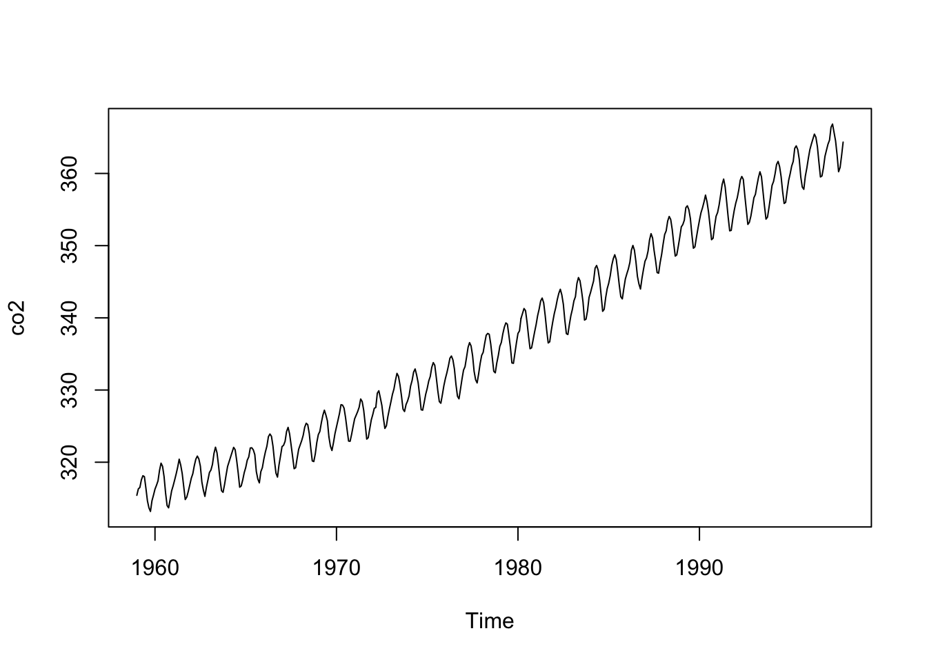
plot(as.numeric(co2))
See the difference? The first one actually calls the function
plot.tsNotice all the plot functions that start with plot.
The function plot will call different functions depending on the class of the arguments:
plotfunction (x, y, ...)
UseMethod("plot")
<bytecode: 0x1157ebb90>
<environment: namespace:base>4.19 Exercises
- What is the sum of the first 100 positive integers? The formula for the sum of integers \(1\) through \(n\) is \(n(n+1)/2\). Define \(n=100\) and then use R to compute the sum of \(1\) through \(100\) using the formula. What is the sum?
n <- 100
n*(n + 1) / 2
[1] 5050- Now use the same formula to compute the sum of the integers from 1 through 1,000.
n <- 1000
n*(n + 1) / 2
[1] 500500- Now use the functions
seqandsumto compute the sum with R for anyn, rather than a formula.
n <- 100
x <- seq(1, 100)
sum(x)
[1] 5050- In math and programming, we say that we evaluate a function when we replace the argument with a given number. So if we type
sqrt(4), we evaluate thesqrtfunction. In R, you can evaluate a function inside another function. The evaluations happen from the inside out. Use one line of code to compute the log, in base 10, of the square root of 100.
log(sqrt(100), base = 10)[1] 1log10(sqrt(100))[1] 1- Make sure the US murders dataset is loaded. Use the function
strto examine the structure of themurdersobject. What are the column names used by the data frame for these five variables?
library(dslabs)
str(murders)
'data.frame': 51 obs. of 5 variables:
$ state : chr "Alabama" "Alaska" "Arizona" "Arkansas" ...
$ abb : chr "AL" "AK" "AZ" "AR" ...
$ region : Factor w/ 4 levels "Northeast","South",..: 2 4 4 2 4 4 1 2 2 2 ...
$ population: num 4779736 710231 6392017 2915918 37253956 ...
$ total : num 135 19 232 93 1257 ...