Distance
Keywords
High dimensional data
Distance
Many of the analyses we perform with high-dimensional data relate directly or indirectly to distance.
Many machine learning techniques rely on defining distances between observations.
Clustering algorithms search of observations that are similar.
But what does this mean mathematically?
The norm
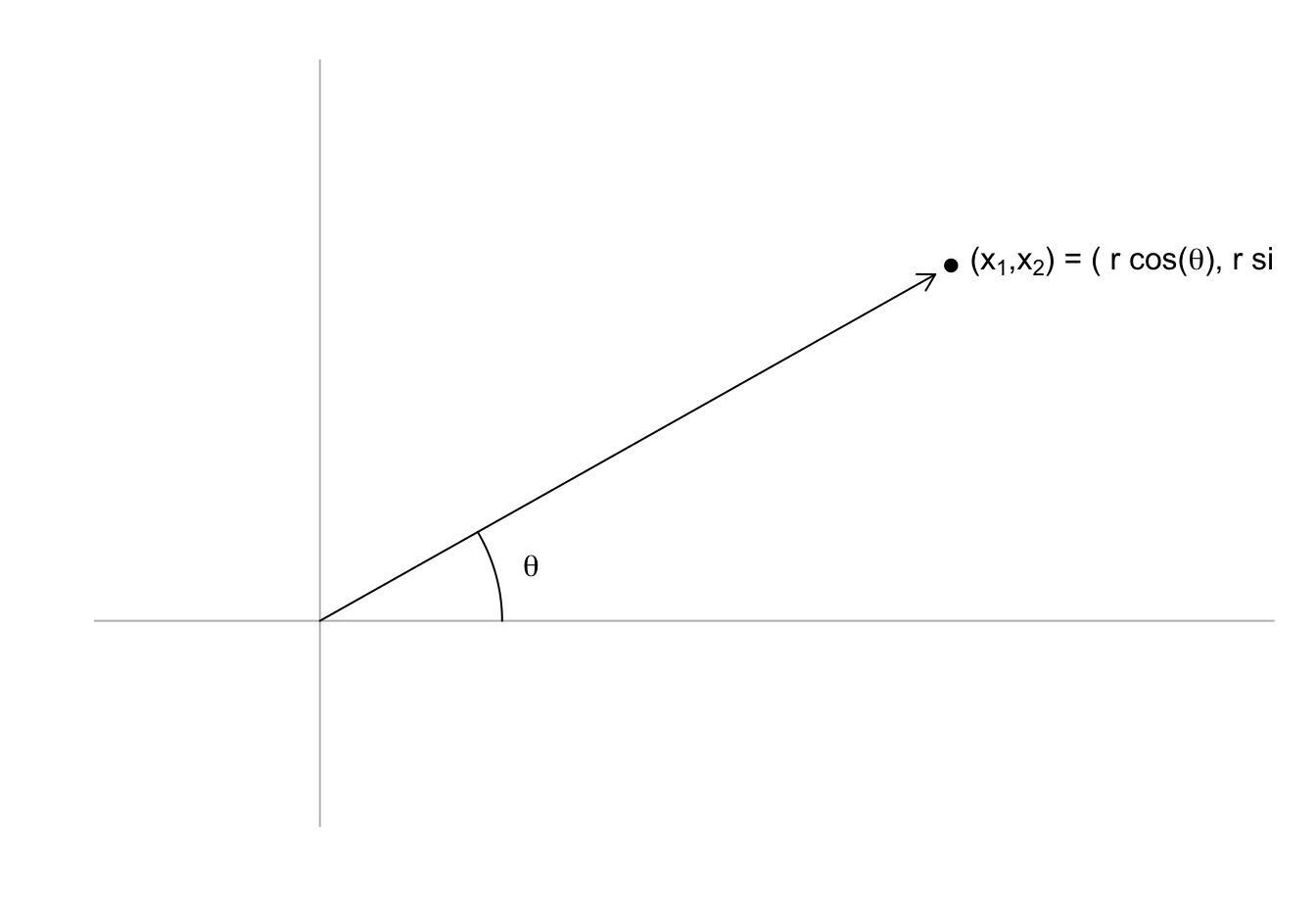
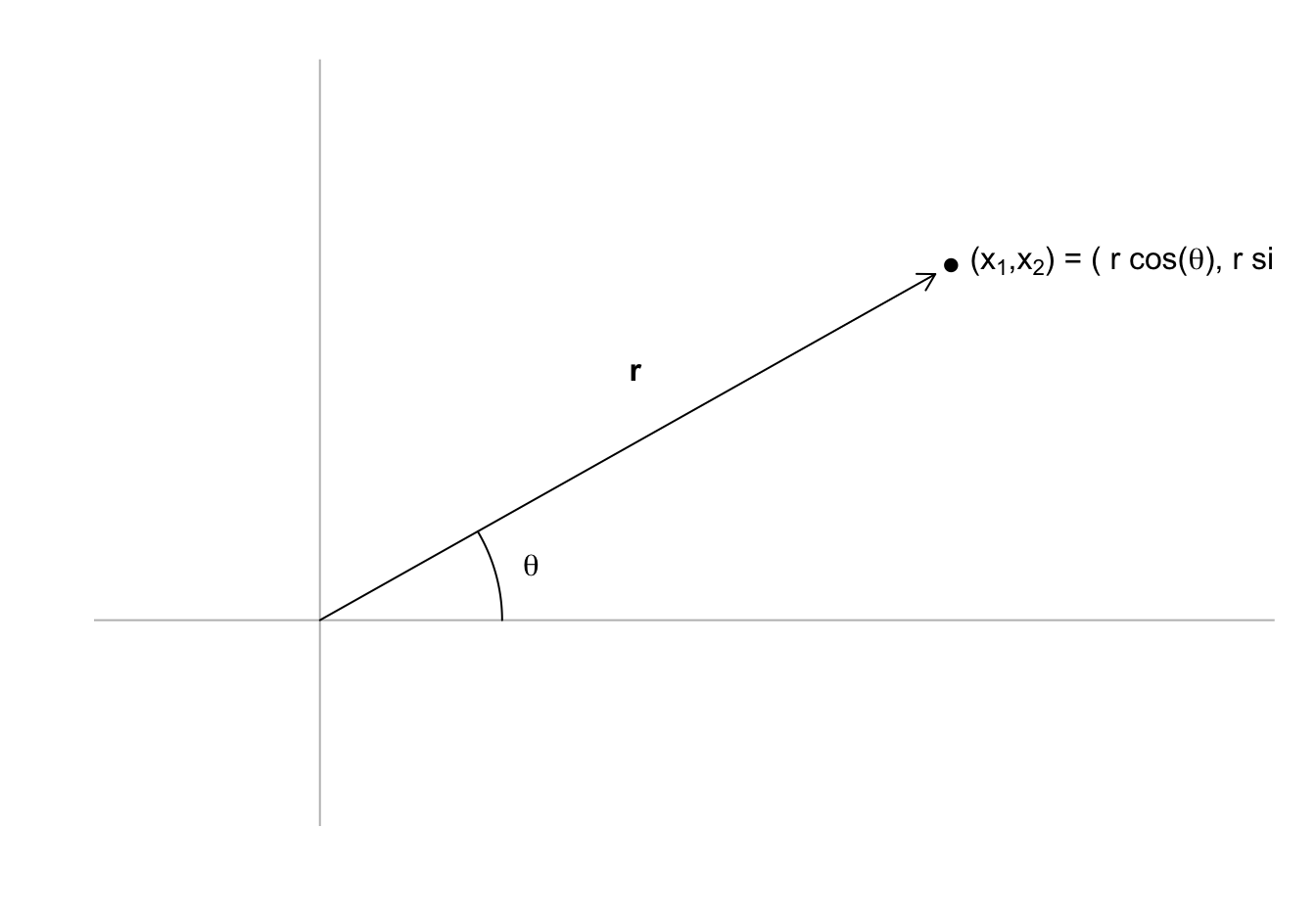
- A point can be represented in polar coordinates:
The norm
- If \(\mathbf{x} = (x_1, x_2)^\top\), \(r\) defines the norm of \(\mathbf{x}\).
The norm
The point of defining the norm is to extrapolate the concept of size to higher dimensions.
Specifically, we write the norm for any vector \(\mathbf{x}\) as:
\[ ||\mathbf{x}|| = \sqrt{x_1^2 + x_2^2 + \dots + x_p^2} \]
- Sometimes convenient to write like this:
\[ ||\mathbf{x}||^2 = x_1^2 + x_2^2 + \dots + x_p^2 \]
The norm
- We define the norm like this:
\[ ||\mathbf{x}||^2 = \mathbf{x}^\top\mathbf{x} \]
Distance
- Distance is the norm of the difference:
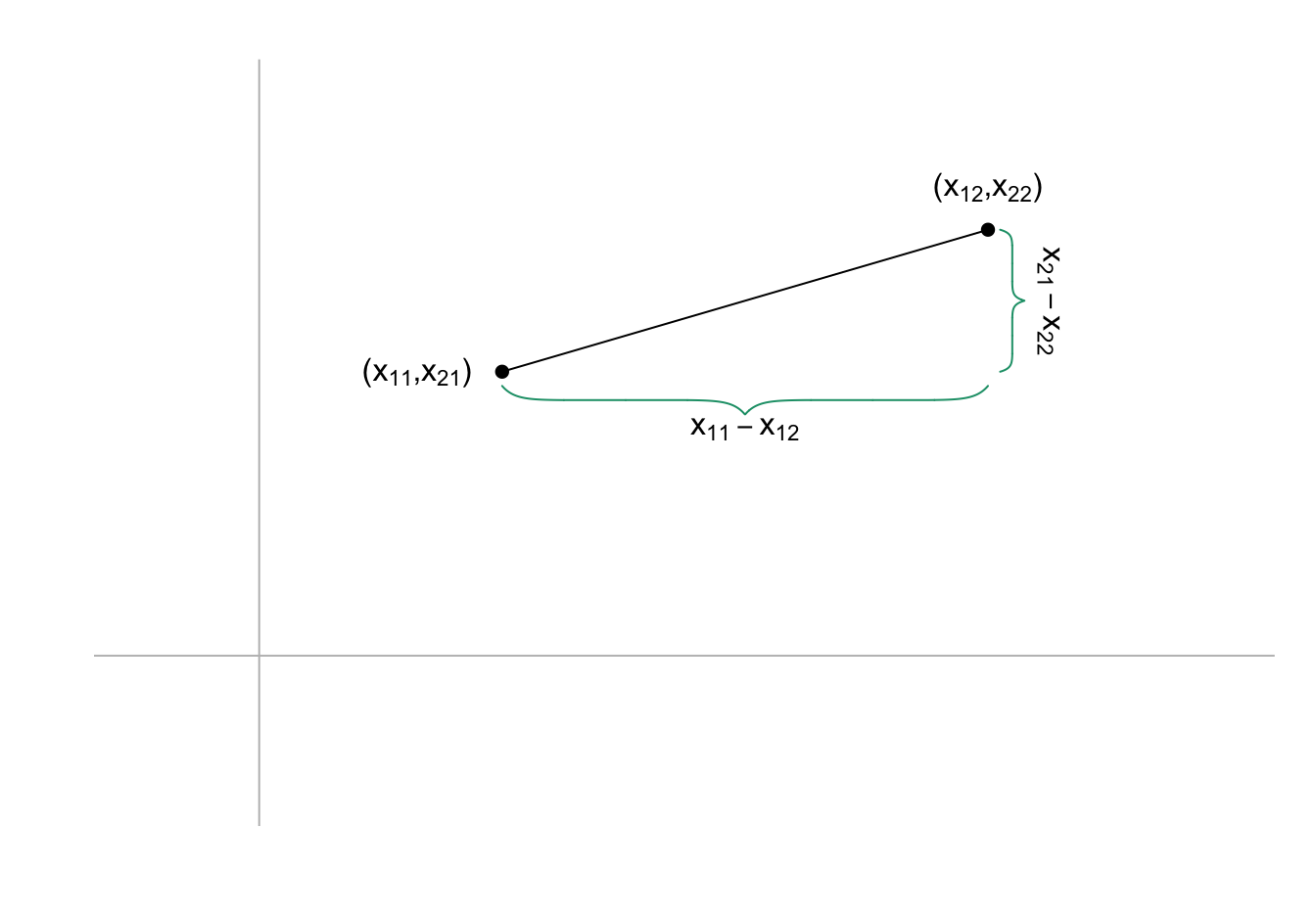
Distance
-We can see this using the definition we know:
\[ \mbox{distance} = \sqrt{(x_{11} - x_{12})^2 + (x_{21} - x_{22})^2} \]
Distance
- Using the norm definition can be extrapolated to any dimension:
\[ \mbox{distance} = || \mathbf{x}_1 - \mathbf{x}_2|| \]
Distance
- For example, the distance between the first and second observation will compute distance using all 784 features:
\[ || \mathbf{x}_1 - \mathbf{x}_2 ||^2 = \sum_{j=1}^{784} (x_{1,j}-x_{2,j })^2 \]
Distance
- Define the features and labels:
mnist <- read_mnist()
x <- mnist$train$images
y <- mnist$train$labels
x_1 <- x[6,]
x_2 <- x[17,]
x_3 <- x[16,] - Compute the distances:
c(sum((x_1 - x_2)^2), sum((x_1 - x_3)^2), sum((x_2 - x_3)^2)) |> sqrt() [1] 2319.867 2331.210 2518.969- Checks out:
y[c(6,17,16)][1] 2 2 7Distance
In R, the function
crossprod(x)is convenient for computing norms.It multiplies
t(x)byx:
c(crossprod(x_1 - x_2), crossprod(x_1 - x_3), crossprod(x_2 - x_3)) |> sqrt() [1] 2319.867 2331.210 2518.969Distance
- We can also compute all the distances at once:
d <- dist(x[c(6,17,16),])
d
1 2
2 2319.867
3 2331.210 2518.969distproduces an object of classdist
class(d) [1] "dist"- There are several machine learning related functions in R that take objects of class
distas input.
Distance
distobjects are similar but not equal to a matrices.To access the entries using row and column indices, we need to coerce it into a matrix.
as.matrix(d)[2,3][1] 2518.969Distance
- The
imagefunction allows us to quickly see an image of distances between observations.
d <- dist(x[1:300,])
image(as.matrix(d)) 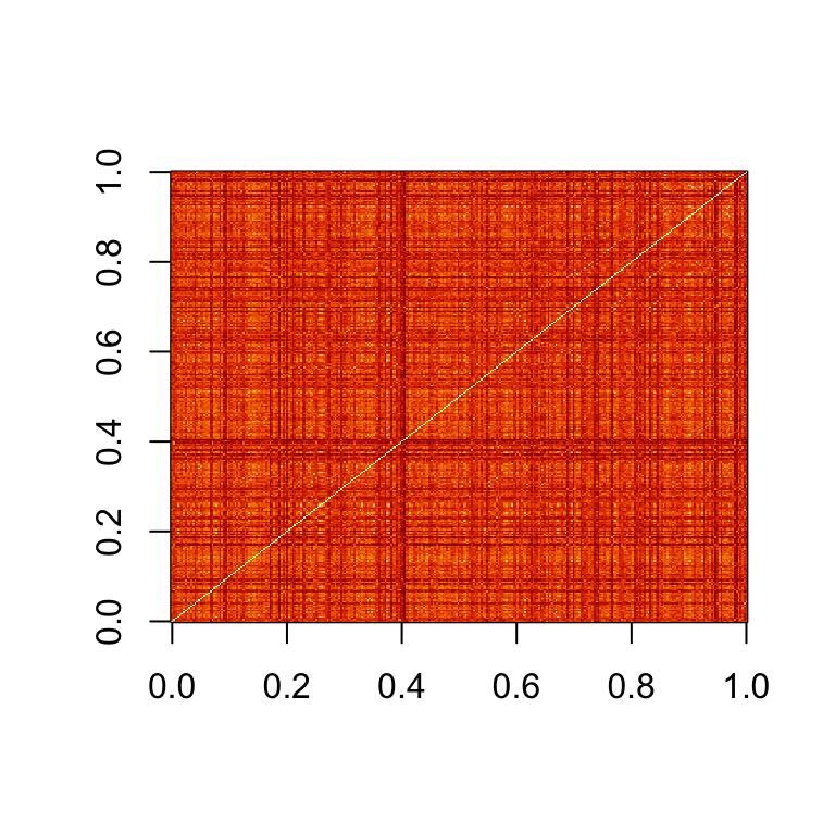
Distance
- If we order distance by the labels:
image(as.matrix(d)[order(y[1:300]), order(y[1:300])]) 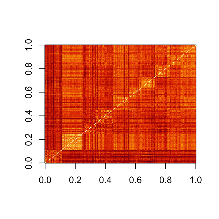
Spaces
Predictor space is a concept that is often used to describe machine learning algorithms.
We can think of all predictors \((x_{i,1}, \dots, x_{i,p})^\top\) for all observations \(i=1,\dots,n\) as \(n\) \(p\)-dimensional points.
The space is the collection of all possible points that should be considered for the data analysis in question, including points we have not observed yet.
In the case of the handwritten digits, we can think of the predictor space as any point \((x_{1}, \dots, x_{p})^\top\) as long as each entry \(x_i, \, i = 1, \dots, p\) is between 0 and 255.
Spaces
Some Machine Learning algorithms also define subspaces.
A commonly defined subspace in machine learning are neighborhoods composed of points that are close to a predetermined center.
We do this by selecting a center \(\mathbf{x}_0\), a minimum distance \(r\), and defining the subspace as the collection of points \(\mathbf{x}\) that satisfy:
\[ || \mathbf{x} - \mathbf{x}_0 || \leq r. \]
Spaces
We can think of this subspace as a multidimensional sphere since every point is the same distance away from the center.
Other machine learning algorithms partition the predictor space into non-overlapping regions and then make different predictions for each region using the data in the region.