R Basics

2025-09-15

Packages

R has a base installation and then tens of thousands of add-on software packages that can be obtained from CRAN
Use install.packages to install the dslabs package from CRAN
Try out the following functions: sessionInfo, installed.packages

Prebuilt functions

Much of what we do in R uses functions from either base R or installed packages.
Many are included in automatically loaded packages: stats, graphics, grDevices, utils, datasets, methods.
This subset of the R universe is referred to as R base.
Very popular packages not included in R base: ggplot2, dplyr, tidyr, and data.table.
It is easy to write your own functions and packages

Important

For problem set 2 you can only use R base.

Base R functions

Example functions that we will use today: ls, rm, library, search, factor, list, exists, str, typeof, and class.
You can see the raw code for a function by typing its name without the parentheses.
- type ls on your console to see an example.

Help system

In R you can use ? or help to learn more about functions.
You can learn about function using

help("ls")

?ls

many packages provide vignettes that are like how-to manuals that can show how the functions in the package are meant to be used to create different analyses

The workspace

Define a variable.

a <- 2

Use ls to see if it’s there. Also take a look at the Environment tab in RStudio.

ls()

[1] "a"

Use rm to remove the variable you defined.

rm(a)

The workspace

each time you start R you will get a new workspace that does not have any variables or libraries loaded
when you quit R you will be asked if you want to save the workspace
- you will probably always be better off saying NO
if you do save a workspace it will be saved as a hidden file (Unix lecture) and whenever R is started in a directory with a saved workspace then that workspace will be re-instantiated and used
- this might be helpful if you are working on a long complex analysis with large data
mostly it is much easier to just use a markdown document to detail your steps and rerun them on a clean workspace
- this can also help find errors in your analysis

The Workspace

just like Unix R uses a search path to find functions that you can evaluate

search()

[1] ".GlobalEnv"        "package:stats"     "package:graphics" 
[4] "package:grDevices" "package:utils"     "package:datasets" 
[7] "package:methods"   "Autoloads"         "package:base"

Variable name convention

A nice convention to follow is to use meaningful words that describe what is stored, only lower case, and underscores as a substitute for spaces.
R and RStudio both provide autocomplete capabilities so you don’t need to type the whole name
- this makes it easier to use longer, more descriptive variable names
It is highly recommended that you not use the period . in variable names, there are situations where R treats it differently and those can cause unintended actions
For more we recommend this guide.

Data types

The main data types in R are:

One dimensional vectors: double, integer, logical, complex, characters.
integer and double are both numeric
Factors
Lists: this includes data frames.
Arrays: Matrices are the most widely used.
Date and time
tibble
S4 objects

Data types

Many errors in R come from confusing data types.
str stands for structure, gives us information about an object.
typeof gives you the basic data type of the object. It reveals the lower-level, more fundamental type of an object in R’s memory.
class This function returns the class attribute of an object. The class of an object is essentially type_of at a higher, often user-facing level.

Data types

Let’s see some example:

library(dslabs)
typeof(murders)

[1] "list"

class(murders)

[1] "data.frame"

str(murders)

'data.frame':   51 obs. of  5 variables:
 $ state     : chr  "Alabama" "Alaska" "Arizona" "Arkansas" ...
 $ abb       : chr  "AL" "AK" "AZ" "AR" ...
 $ region    : Factor w/ 4 levels "Northeast","South",..: 2 4 4 2 4 4 1 2 2 2 ...
 $ population: num  4779736 710231 6392017 2915918 37253956 ...
 $ total     : num  135 19 232 93 1257 ...

dim(murders)

[1] 51  5

Data frames

Date frames are the most common class used in data analysis.
Data frames are like a matrix, but where the columns can have different types.
Usually, rows represents observations and columns variables.
you can index them like you would a matrix, x[i, j] refers to the element in row i column j
You can see part of the content like this

head(murders)

       state abb region population total
1    Alabama  AL  South    4779736   135
2     Alaska  AK   West     710231    19
3    Arizona  AZ   West    6392017   232
4   Arkansas  AR  South    2915918    93
5 California  CA   West   37253956  1257
6   Colorado  CO   West    5029196    65

Data frames

and you can use View to open a spreadsheet-like interface to see the entire data.frame.

View(murders)

This is more effective in RStudio because it has an integrated viewer.

Data frames

A very common operation is adding columns like this:

murders$pop_rank <- rank(murders$population)
head(murders)

       state abb region population total pop_rank
1    Alabama  AL  South    4779736   135       29
2     Alaska  AK   West     710231    19        5
3    Arizona  AZ   West    6392017   232       36
4   Arkansas  AR  South    2915918    93       20
5 California  CA   West   37253956  1257       51
6   Colorado  CO   West    5029196    65       30

Data frames

Note that we used the $.
This is called an accessor because it lets us access columns.

murders$population

 [1]  4779736   710231  6392017  2915918 37253956  5029196  3574097   897934
 [9]   601723 19687653  9920000  1360301  1567582 12830632  6483802  3046355
[17]  2853118  4339367  4533372  1328361  5773552  6547629  9883640  5303925
[25]  2967297  5988927   989415  1826341  2700551  1316470  8791894  2059179
[33] 19378102  9535483   672591 11536504  3751351  3831074 12702379  1052567
[41]  4625364   814180  6346105 25145561  2763885   625741  8001024  6724540
[49]  1852994  5686986   563626

More generally: $ can be used to access named components of a list.

Data frames

One way R confuses beginners is by having multiple ways of doing the same thing.
For example you can access the 4th column in the following five different ways:

murders$population
murders[, "population"]
murders[, 4]
murders[["population"]]
murders[[4]]

In general, we recommend using the name rather than the number as adding or removing columns will change index values, but not names.

with

with let’s us use the column names as symbols to access the data.
This is convenient to avoid typing the data frame name over and over:

rate <- with(murders, total/population)

with

Note you can write entire code chunks by enclosing it in curly brackets:

with(murders, {
   rate <- total/population
   rate <- round(rate*10^5)
   print(rate[1:5])
})

[1] 3 3 4 3 3

Vectors

The columns of data frames are an example of one dimensional (atomic) vectors.
An atomic vector is a vector where every element must be the same type.

length(murders$population)

[1] 51

typeof(murders$population)

[1] "double"

Vectors

Often we have to create vectors.
The concatenate function c is the most basic way used to create vectors:

x <- c("b", "s", "t", " ", "2", "6", "0")

We access the elements using []

x[5]

[1] "2"

typeof(x[5])

[1] "character"

x[12]

[1] NA

NOTE R does not do array bounds checking…it silently pads with missing values

Sequences

Sequences are a common example of vectors we generate.

seq(1, 10)

 [1]  1  2  3  4  5  6  7  8  9 10

seq(1, 9, by=2)

[1] 1 3 5 7 9

When you want a sequence that increases by 1 you can use the colon :

1:10

 [1]  1  2  3  4  5  6  7  8  9 10

3.3:7.8

[1] 3.3 4.3 5.3 6.3 7.3

4:-1

[1]  4  3  2  1  0 -1

Sequences

A useful function to quickly generate a sequence the same length as a vector x is seq_along(x) and NOT 1:length(x)

x <- c("b", "s", "t", " ", "2", "6", "0")
seq_along(x)

[1] 1 2 3 4 5 6 7

A reason to use this is to loop through entries:

for (i in seq_along(x)) {
  cat(toupper(x[i]))
}

BST 260

But if the length of x is zero, then using 1:length(x) does not work for this loop

w = x[x=="W"]
1:length(w)

[1] 1 0

seq_along(w)

integer(0)

Vector types and coercion

One dimensional vectors: double, integer, logical, complex, characters and numeric
Each basic type has its own version of NA (a missing value)
testing for types: is.TYPE,
coercing : as.TYPE, will result in NA if it is not possible

is.numeric("a")

[1] FALSE

is.double(1L)

[1] FALSE

as.double("6")

[1] 6

as.numeric(x) + 3

[1] NA NA NA NA  5  9  3

typeof(1:10)

[1] "integer"

Coercing

When you do something inconsistent with data types, R tries to figure out what you mean and change it accordingly.
We call this coercing.
R does not return an error and in some cases does not return a warning either.
This can cause confusion and unnoticed errors.
So it’s important to understand how and when it happens.

Vector types and coercion

coercion is automatically performed when it is possible
TRUE coerces to 1 and FALSE to 0
but any non-zero integer coerces to TRUE, only 0 coerces to FALSE
as.logical converts 0 and only 0 to FALSE, everything else to TRUE
the character string “NA” is not a missing value

typeof(1:10 + 0.1)

[1] "double"

typeof(TRUE+1)

[1] "double"

as.character(TRUE)

[1] "TRUE"

as.numeric(TRUE)

[1] 1

as.logical(1)

[1] TRUE

as.logical(.5)

[1] TRUE

Coercing

Here are some examples:

typeof(1L)

[1] "integer"

typeof(1)

[1] "double"

typeof(1 + 1L)

[1] "double"

c("a", 1, 2)

[1] "a" "1" "2"

TRUE + FALSE

[1] 1

factor("a") == "a"

[1] TRUE

identical(factor("a"), "a")

[1] FALSE

Coercing

When R can’t figure out how to coerce, rather an error it returns an NA:

as.numeric("a")

[1] NA

Note that including NAs in arithmetical operations usually returns an NA.

1 + 2 + NA

[1] NA

Coercing

You can coerce explicitly
Most coercion functions start with as.
Here is an example.

x <- factor(c("a","b","b","c"))
as.character(x)

[1] "a" "b" "b" "c"

as.numeric(x)

[1] 1 2 2 3

Coercing

The readr package provides some tools for trying to par

x <- c("12323", "12,323")
as.numeric(x)

[1] 12323    NA

library(readr)
parse_guess(x)

[1] 12323 12323

Factors

One key distinction between data types you need to understad is the difference between factors and characters.
The murder dataset has examples of both.

class(murders$state)

[1] "character"

class(murders$region)

[1] "factor"

Why do you think this is?

Factors

A factor is a good representation for a variable, that has a fixed set of non-numeric values
- ex: Sex has Male and Female
It is usually not a good representation for variables that have lots of levels (like state names in the murders dataset)
Internally a factor is stored as the unique set of labels (called levels) and an integer vector with values in 1 to length(levels)
- if the ith entry is k then that corresponds to the kth element of the levels
In statistics we refer to this as categorical data, where all of the individuals are mapped into a relatively small number of categories.
Usually order does not matter, but if it does you can also have ordered factors.

x <- murders$region
levels(x)

[1] "Northeast"     "South"         "North Central" "West"

Setting Levels

you can set up the levels as you would like, when creating a factor
if you do not set them up, then they will be created in lexicographic order (in the locale you are using)

x = sample(c("Male", "Female"), 50, replace =TRUE)
y1 = factor(x, levels=c("Male", "Female"))
y2 = factor(x, levels = c("Female", "Male"))
y1[1:10]

 [1] Female Male   Female Male   Female Female Female Female Male   Female
Levels: Male Female

y2[1:10]

 [1] Female Male   Female Male   Female Female Female Female Male   Female
Levels: Female Male

Categories based on strata

In data analysis we often want to stratify continuous variables into categories.
The function cut helps us do this:
In this case there may be a reason to think of using ordered factors.

age <- c(5, 93, 18, 102, 14, 22, 45, 65, 67, 25, 30, 16, 21)
cut(age, c(0, 11, 27, 43, 59, 78, 96, Inf))

 [1] (0,11]   (78,96]  (11,27]  (96,Inf] (11,27]  (11,27]  (43,59]  (59,78] 
 [9] (59,78]  (11,27]  (27,43]  (11,27]  (11,27] 
Levels: (0,11] (11,27] (27,43] (43,59] (59,78] (78,96] (96,Inf]

Categories based on strata

We can assign more meaningful level names:

age <- c(5, 93, 18, 102, 14, 22, 45, 65, 67, 25, 30, 16, 21)
cut(age, c(0, 11, 27, 43, 59, 78, 96, Inf), 
    labels = c("Alpha", "Zoomer", "Millennial", "X", "Boomer", "Silent", "Greatest"))

 [1] Alpha      Silent     Zoomer     Greatest   Zoomer     Zoomer    
 [7] X          Boomer     Boomer     Zoomer     Millennial Zoomer    
[13] Zoomer    
Levels: Alpha Zoomer Millennial X Boomer Silent Greatest

Changing levels

This is often needed for ordinal data because R defaults to alphabetical order
Or as noted you may want to make use of ordered factors

gen <- factor(c("Alpha", "Zoomer", "Millennial"))
levels(gen)

[1] "Alpha"      "Millennial" "Zoomer"

You can change this with the levels argument:

gen <- factor(gen, levels = c("Alpha", "Zoomer", "Millennial", "X", "Boomer", "Silent", "Greatest"))
levels(gen)

[1] "Alpha"      "Zoomer"     "Millennial" "X"          "Boomer"    
[6] "Silent"     "Greatest"

Changing levels

A common reason we want to change levels is to assure R is aware which is the reference strata.
This is important for linear models because the first level is assumed to be the reference.

x <- factor(c("no drug", "drug 1", "drug 2"))
levels(x)

[1] "drug 1"  "drug 2"  "no drug"

x <- relevel(x, ref = "no drug")
levels(x)

[1] "no drug" "drug 1"  "drug 2"

Changing levels

We often want to order strata based on a summary statistic.
This is common in data visualization.
We can use reorder for this:

x <- reorder(murders$region, murders$population, sum)

Factors

Another reason we used factors is because they are stored more efficiently:

x <- sample(murders$state[c(5,33,44)], 10^7, replace = TRUE)
y <- factor(x)
object.size(x)

80000232 bytes

object.size(y)

40000648 bytes

An integer uses less memory than a character string (but it is a bit more complicated)

Factors can be confusing

Try to make sense of this:

x <- factor(c("3","2","1"), levels = c("3","2","1"))
as.numeric(x)

[1] 1 2 3

x[1]

[1] 3
Levels: 3 2 1

levels(x[1])

[1] "3" "2" "1"

table(x[1])


3 2 1 
1 0 0

Factors can be confusing

Avoid keeping extra levels with droplevels:

z <- x[1]
z <- droplevels(z)

But note what happens if we change to another level:

z[1] <- "1"
z

[1] <NA>
Levels: 3

NAs

NA stands for not available and represents data that are missing.
Data analysts have to deal with NAs often.
In R there is a different kind of NA for each of the basic vector data types.
There is also the concept of NULL, which represents a zero length list and is often returned by functions or expressions that do not have a specified return value

NAs

dslabs includes an example dataset with NAs

library(dslabs)
na_example[1:20]

 [1]  2  1  3  2  1  3  1  4  3  2  2 NA  2  2  1  4 NA  1  1  2

The is.na function is key for dealing with NAs

is.na(na_example[1])

[1] FALSE

is.na(na_example[17])

[1] TRUE

is.na(NA)

[1] TRUE

is.na("NA")

[1] FALSE

NAs

Caution logical operators like and (&) and or (|) coerce their arguments when needed and possible
the logical operators evaluate arguments in a “lazy” fashion, and left to right

TRUE & NA

[1] NA

TRUE & 0

[1] FALSE

TRUE | NA

[1] TRUE

NaNs and Inf

A related constant is NaN which stands for Not a Number
NaN is a double, coercing it to integer yields an NA
Inf and -Inf represent values of infinity and minus infinity (RStudio makes using these really annoying)

0/0

[1] NaN

class(0/0)

[1] "numeric"

sqrt(-1)

[1] NaN

log(-1)

[1] NaN

1/Inf

[1] 0

Inf-Inf

[1] NaN

Lists

Data frames are a type of list.
Lists permit components of different types and, unlike data frames, different lengths:

x <- list(name = "John", id = 112, grades = c(95, 87, 92))

The JSON format is best represented as list in R.

Lists

You can access components in different ways:

x$name

[1] "John"

x[[1]]

[1] "John"

x[["name"]]

[1] "John"

Matrices

Matrices are another widely used data type.
They are similar to data frames except all entries need to be of the same type.
We will learn more about matrices in the High Dimensional Data Analysis part of the class.

Functions

You can define your own function. The form is like this:

f <- function(x, y, z = 0){
  ### do calculations with x, y, z to compute object
  return(object)
}

the values you pass to the function are called the arguments and they can have default values (e.g above z is 0 unless provided)
arguments are matched by either name (which takes precedence) or position
the value returned by a function is either the value specified in a call to return or the value of the last statement evaluated

Functions

Here is an example of a function that sums $1,2,\dots,n$
within the body of a function the arguments are referred to by their symbols and they take the value supplied at the time of invocation
any symbol found in the body of the function that does not match an argument has to be matched to a value by a process called scoping

s <- function(n){
   return(sum(1:n))
}

Flow-control and operators

R has all the standard flow control constructs that most computer langagues do
if/else; while; repeat; for; break; next
you can read the manual pages by calling help or using ? (but for the latter you must quote the argument)

 help("for")
 ?"break"
 ?"&"
 ?"/"

Logical Operators

the short forms & and | perform element-wise comparisons (vectorized)
the long forms && and || evaluate the first element only, move left to right and return when the result is determined
errors often occur when a programmer/analyst uses one form, when they want the other (R tries to warn you when it thinks there is a mistake)

Arithmetic Operators

these are operators like ^ or +
?Syntax will get you the manual page for operator precedence
when in doubt always use parentheses - it is much clearer to the reader

2^1+1

[1] 3

2^(1+1)

[1] 4

TRUE || TRUE && FALSE   # is the same as

[1] TRUE

TRUE || (TRUE && FALSE) # and different from

[1] TRUE

(TRUE || TRUE) && FALSE

[1] FALSE

Functions

in R functions are first class objects - this means they can be passed as arguments, assigned to symbols, stored in other data structures
in particular they can be passed as arguments to a function and returned as values
in some languages (e.g. C or Java) functions are not first class objects and they cannot be passed as arguments
Python uses a fairly similar strategy for functions to the one used in R (as do many other languages)

Scope

most of what computer languages do is map symbols (syntax) to values (semantics) and then create an executable program
when a computer comes upon an expression it parses it and that identifies the symbols that will need to be looked up

expr <- parse(text = "a + b * c")
expr[[1]][1]

`+`()

expr[[1]][2]

a()

expr[[1]][3]

(b * c)()

the third part itself is a compound expression that can be decomposed into its parts, *, b and c
in order to evaluate this the evaluator must find bindings for each of the symbols
here we expect it wants numbers for a, b and c and functions for + and *

##Scope

all computer languages have a set of rules that are used to match these symbols to values
one commonly used rule is to use lexical scope, but there are lots of different ways this is done

fun1 = function(x)  x + y
fun1(4)

in fun1(4) we probably all agree that the value that should be used for x is 4, we probably expect that + is a system function
but what about y - where should it’s value come from?

Scope

Read the function below and try to understand what happens when it is evaluated:

f <- function(x){
  cat("y is", y,"\n")
  y <- x
  cat("y is", y,"\n")
  return(y)
}
y <- 2
f(3)

y is 2 
y is 3

[1] 3

Lexical Scope

lexical scope says that for any function with unbound values you should use the environment at the time the function was created to first look for bindings, in R (and Python) after that you look in the global environment (your workspace) and then in attached packages and system functions.
why is this useful?

Lexical Scope

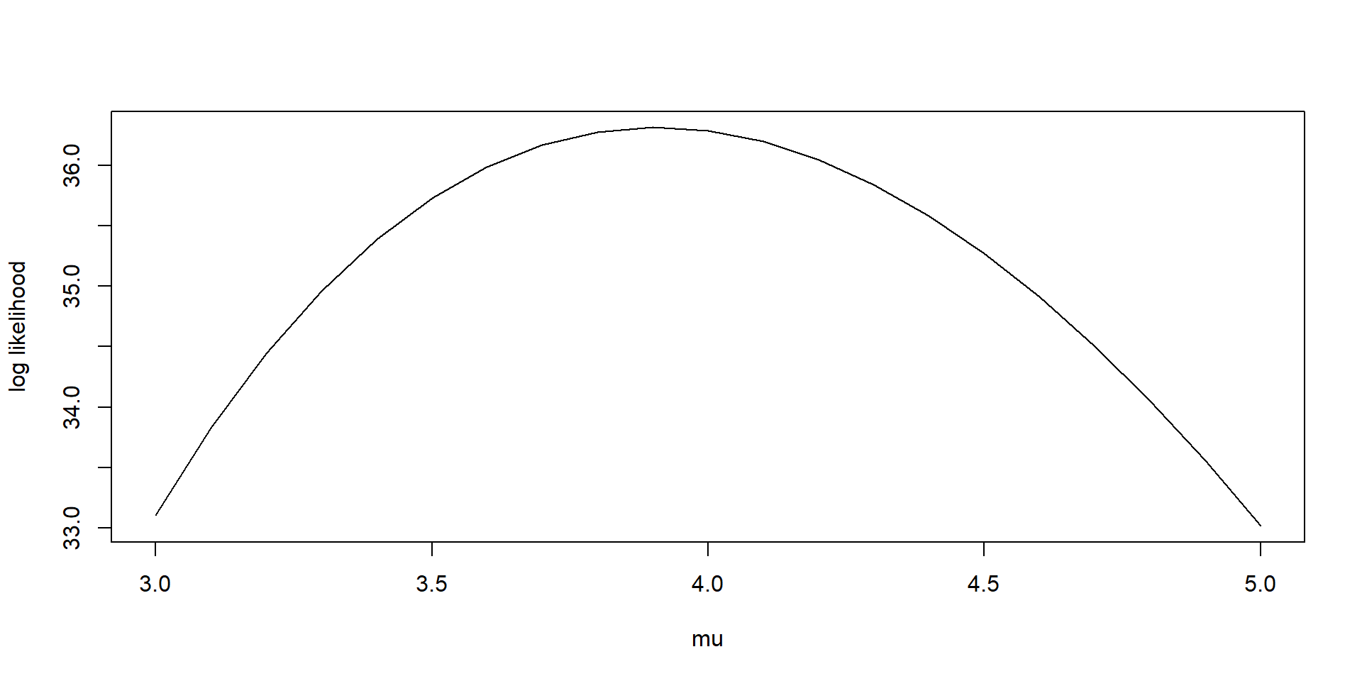
we can write some interesting functions - like a function that evaluates the log likelihood for any given set of data
here we use rexp to generate values from an Exponential distribution
notice that a function is returned and that R notes that it is a closure

x = rexp(100, rate = 4)

llExp = function(DATA) {
   n = length(DATA)
   sumx = sum(DATA)
   return(function(mu) {n * log(mu) - mu * sumx})
}

myLL = llExp(x)
myLL

function (mu) 
{
    n * log(mu) - mu * sumx
}
<environment: 0x000001b09f72caf8>

Lexical Scope Example

here we generate different potential values for the rate parameter and plot the log likelihood - the MLE is the maximum of this

##possible values for mu
y = seq(3,5,by = 0.1)

plot(y, myLL(y), type="l", xlab="mu", ylab="log likelihood")

Name collisions

what happens when authors of two different packages choose the same name for their functions?
Look at how this function associated with the symbol filter changes in the following code segment:

filter
library(dplyr)
filter

by calling library(dplyr) a new package has been put on the search list. You can call search() before and after the call to library
one implication of this observation is that users could inadvertently alter computations - and we will want to protect against that

Evaluation and the process used to find bindings

when evaluating a function R first establishes an evaluation environment that contains the formal arguments matched to the supplied arguments
if the function is in a package, then the Namespace directives of the package are used to augment this evaluation environment
any symbol not found in that evaluation environment will be searched for in the Global Environment (your workspace).
And after that the search path (search()) in order.
The evaluator will take the first match it finds and try to use that (sort of - it does know when it is looking for a function)

Namespaces

when authoring a package you will want to use Namespaces - the details will not be discussed here
If a package uses a Namespace then you can explicitly say which filter you want using :::

stats::filter
dplyr::filter

Examples

Restart your R Console and study this example:

library(dslabs)
exists("murders")

[1] TRUE

murders <- murders
murders2 <- murders
rm(murders)
exists("murders")

[1] TRUE

detach("package:dslabs")
exists("murders")

[1] FALSE

exists("murders2")

[1] TRUE

Object Oriented Programming

R uses object oriented programming (OOP).
Base R uses two approaches referred to as S3 and S4, respectively.
S3, the original approach, is more common, but has some severe limitations
The S4 approach is more similar to the conventions used by the Lisp family of languages.
In S4 there are classes that are used to describe data structures and generic functions, that have methods associated with them

plot(co2)

plot(as.numeric(co2))

Object Oriented Programming

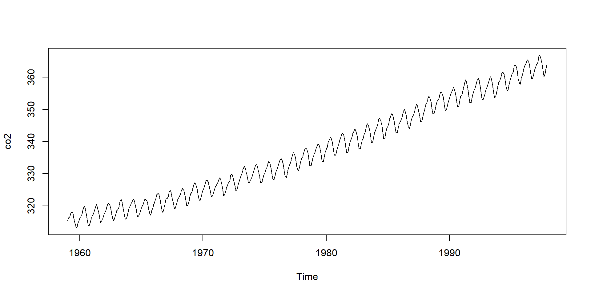
Note co2 is not numeric:

class(co2)

[1] "ts"

The plots are different because plot behaves differently with different classes.

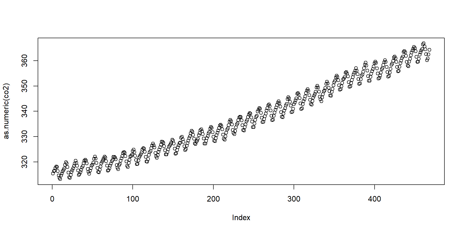
Object Oriented Programming

The first plot actually calls the function

plot.ts

Notice all the plot functions that start with plot by typing plot. and then tab.
The function plot will call different functions depending on the class of the arguments.

Plots

Soon we will learn how to use the ggplot2 package to make plots.
R base does have functions for plotting though
Some you should know about are:
- plot - mainly for making scatterplots.
- lines - add lines/curves to an existing plot.
- hist - to make a histogram.
- boxplot - makes boxplots.
- image - uses color to represent entries in a matrix.

Plots

Although, in general, we recommend using ggplot2, R base plots are often better for quick exploratory plots.
For example, to make a histogram of values in x simply type:

hist(x)

To make a scatter plot of y versus x and then interpolate we type:

plot(x,y)
lines(x,y)

R Basics

Packages

Prebuilt functions

Base R functions

Help system

The workspace

The workspace

The Workspace

Variable name convention

Data types

Data types

Data types

Data frames

Data frames

Data frames

Data frames

Data frames

with

with

Vectors

Vectors

Sequences

Sequences

Vector types and coercion

Coercing

Vector types and coercion

Coercing

Coercing

Coercing

Coercing

Factors

Factors

Setting Levels

Categories based on strata

Categories based on strata

Changing levels

Changing levels

Changing levels

Factors

Factors can be confusing

Factors can be confusing

NAs

NAs

NAs

NaNs and Inf

Lists

Lists

Matrices

Functions

the value returned by a function is either the value specified in a call to return or the value of the last statement evaluated

Functions

Flow-control and operators

Logical Operators

Arithmetic Operators

Functions

Scope

Scope

Lexical Scope

Lexical Scope

Lexical Scope Example

Name collisions

Evaluation and the process used to find bindings

Namespaces

Examples

Object Oriented Programming

Object Oriented Programming

Object Oriented Programming

Object Oriented Programming

Plots

Plots

the value returned by a function is either the value specified in a call to `return` or the value of the last statement evaluated