Web Scraping
2024-09-30
Scraping HTML
The data we need to answer a question is not always in a spreadsheet ready for us to read.
For example, the US murders dataset we used in the R Basics chapter originally comes from this Wikipedia page:
Scraping HTML
- You can see the data table when you visit the webpage:
 .
.
- Web scraping, or web harvesting, is the term we use to describe the process of extracting data from a website.
Scraping HTML
The reason we can do this is because the information used by a browser to render webpages is received as a text file from a server.
The text is code written in hyper text markup language (HTML).
Every browser has a way to show the html source code for a page, each one different.
On Chrome, you can use Control-U on a PC and command+alt+U on a Mac.
Scraping HTML
 .
.
HTML
Because this code is accessible, we can download the HTML file, import it into R, and then write programs to extract the information we need from the page.
However, once we look at HTML code, this might seem like a daunting task.
But we will show you some convenient tools to facilitate the process.
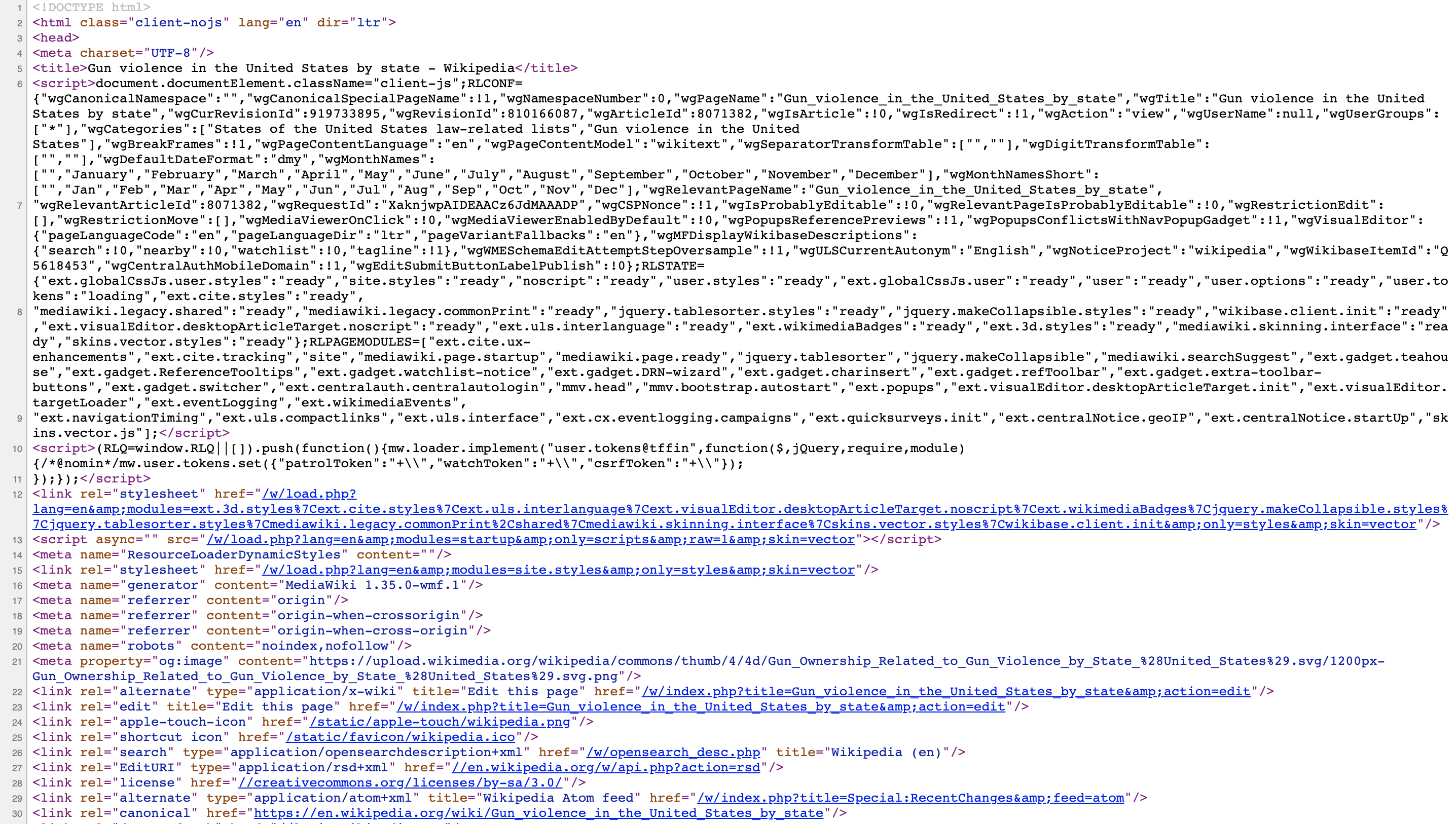
HTML
- To get an idea of how it works, here are a few lines of code from the Wikipedia page that provides the US murders data:
<table class="wikitable sortable">
<tr>
<th>State</th>
<th><a href="/wiki/List_of_U.S._states_and_territories_by_population"
title="List of U.S. states and territories by population">Population</a><br />
<small>(total inhabitants)</small><br />
<small>(2015)</small> <sup id="cite_ref-1" class="reference">
<a href="#cite_note-1">[1]</a></sup></th>
<th>Murders and Nonnegligent
<p>Manslaughter<br />
<small>(total deaths)</small><br />
<small>(2015)</small> <sup id="cite_ref-2" class="reference">
<a href="#cite_note-2">[2]</a></sup></p>
</th>
<th>Murder and Nonnegligent
<p>Manslaughter Rate<br />
<small>(per 100,000 inhabitants)</small><br />
<small>(2015)</small></p>
</th>
</tr>
<tr>
<td><a href="/wiki/Alabama" title="Alabama">Alabama</a></td>
<td>4,853,875</td>
<td>348</td>
<td>7.2</td>
</tr>
<tr>
<td><a href="/wiki/Alaska" title="Alaska">Alaska</a></td>
<td>737,709</td>
<td>59</td>
<td>8.0</td>
</tr>
<tr>
HTML
You can actually see the data, except data values are surrounded by html code such as
<td>.We can also see a pattern of how it is stored.
If you know HTML, you can write programs that leverage knowledge of these patterns to extract what we want.
We also take advantage of a language widely used to make webpages look “pretty” called Cascading Style Sheets (CSS).
HTML
Although we provide tools that make it possible to scrape data without knowing HTML, it is useful to learn some HTML and CSS.
Not only does this improve your scraping skills, but it might come in handy if you are creating a webpage to showcase your work.
There are plenty of online courses and tutorials for learning these.
Two examples are Codeacademy and W3schools.
The rvest package
The tidyverse provides a web harvesting package called rvest.
The first step using this package is to import the webpage into R.
The package makes this quite simple:
- Note that the entire Murders in the US Wikipedia webpage is now contained in
h.
The rvest package
- The class of this object is:
The rvest package is actually more general; it handles XML documents.
XML is a general markup language (that’s what the ML stands for) that can be used to represent any kind of data.
HTML is a specific type of XML specifically developed for representing webpages.
The rvest package
Now, how do we extract the table from the object
h? If you were to printh, we would see information about the object that is not very informative.We can see all the code that defines the downloaded webpage using the
html_textfunction like this:
The rvest package
We don’t show the output here because it includes thousands of characters.
But if we look at it, we can see the data we are after are stored in an HTML table: you can see this in this line of the HTML code above
<table class="wikitable sortable">.
The rvest package
The different parts of an HTML document, often defined with a message in between
<and>are referred to as nodes.The rvest package includes functions to extract nodes of an HTML document:
html_nodesextracts all nodes of different types andhtml_nodeextracts the first one.
The rvest package
- To extract the tables from the html code we use:
- Now, instead of the entire webpage, we just have the html code for the tables in the page:
The rvest package
{xml_nodeset (2)}
[1] <table class="wikitable sortable"><tbody>\n<tr>\n<th>State\n</th>\n<th>\n ...
[2] <table class="nowraplinks hlist mw-collapsible mw-collapsed navbox-inner" ...- The table we are interested is the first one:
The rvest package
This is clearly not a tidy dataset, not even a data frame.
In the code above, you can definitely see a pattern and writing code to extract just the data is very doable.
In fact, rvest includes a function just for converting HTML tables into data frames:
The rvest package
- We can now make the data frame:
tab <- tab |>
  setNames(c("state", "population", "total", "murder_rate")) |>
  mutate(across(c(population, total), parse_number))
head(tab)
# A tibble: 6 × 4
state population total murder_rate
<chr> <dbl> <dbl> <dbl>
1 Alabama 4853875 348 7.2
2 Alaska 737709 59 8
3 Arizona 6817565 309 4.5
4 Arkansas 2977853 181 6.1
5 California 38993940 1861 4.8
6 Colorado 5448819 176 3.2