Foundations of Statistical Inference

2024-10-21

Sampling models

Many data generation procedures can be effectively modeled as draws from an urn.
We can model the process of polling likely voters as drawing 0s for one party and 1s for the other.
Epidemiologist assume subjects in their studies are a random sample from the population of interest.

Sampling models

In general, the data related to a specific outcome can be modeled as a random sample from an urn containing the outcomes for the entire population of interest.

Sampling models

Similarly, in experimental research, we often assume that the individual organisms we are studying, for example worms, flies, or mice, are a random sample from a larger population.
Randomized experiments can be modeled by draws from an urn, reflecting the way individuals are assigned into group; when getting assigned, individuals draw their group at random.

Sampling models

Sampling models are therefore ubiquitous in data science.
Casino games offer a plethora of real-world cases in which sampling models are used to answer specific questions.
We will therefore start with these examples.

Sampling models

Suppose a very small casino hires you to consult on whether they should set up roulette wheels.
We will assume that 1,000 people will play, and that the only game available on the roulette wheel is to bet on red or black.
The casino wants you to predict how much money they will make or lose.
They want a range of values and, in particular, they want to know what’s the chance of losing money.

Sampling models

If this probability is too high, they will decide against installing roulette wheels.
We are going to define a random variable $S$ that will represent the casino’s total winnings.

Sampling models

This is a roullette:

Sampling models

Let’s start by constructing the urn.
A roulette wheel has 18 red pockets, 18 black pockets and 2 green ones.
So playing a color in one game of roulette is equivalent to drawing from this urn:

color <- rep(c("Black", "Red", "Green"), c(18, 18, 2))

Sampling models

The 1,000 outcomes from 1,000 people playing are independent draws from this urn.
If red comes up, the gambler wins, and the casino loses a dollar, resulting random variable being -$1.
Otherwise, the casino wins a dollar, and the random variable is $1.

Sampling models

To construct our random variable $S$, we can use this code:

n <- 1000 
x <- sample(ifelse(color == "Red", -1, 1),  n, replace = TRUE) 
x[1:10] 
#>  [1]  1 -1  1 -1  1  1 -1  1  1  1

Sampling models

Because we know the proportions of 1s and -1s, we can generate the draws without defining color.

x <- sample(c(-1, 1), n, replace = TRUE, prob = c(9/19, 10/19))

Sampling models

This is a sampling model, as it models the random behavior through the sampling of draws from an urn.
The total winnings $S$ is simply the sum of these 1,000 independent draws:

x <- sample(c(-1, 1), n, replace = TRUE, prob = c(9/19, 10/19)) 
s <- sum(x) 
s 
#> [1] 44

If you rerun the code above, you see that $S$ changes every time.
$S$ is a random variable.

The probability distributions

The probability distribution of a random variable informs us about the probability of the observed value falling in any given interval.
For example, if we want to know the probability that we lose money, we are asking the probability that $S$ is in the interval $(-\infty,0)$.

The probability distribution

If we can define a cumulative distribution function $F(a) = \mbox{Pr}(S\leq a)$, we can answer any question about the probability of events defined by $S$.
We call this $F$ the random variable’s distribution function.
Probability and Statistics classes dedicate much time to calculating or approximating these.
We can also estimate the distribution function for $S$ using a Monte Carlo simulation.

The probability distribution

With this code, we run the experiment of having 1,000 people repeatedly play roulette, specifically $B = 10,000$ times:

n <- 1000 
B <- 10000 
roulette_winnings <- function(n){ 
  x <- sample(c(-1, 1), n, replace = TRUE, prob = c(9/19, 10/19)) 
  sum(x) 
} 
s <- replicate(B, roulette_winnings(n))

The probability distribution

Now, we can ask the following: in our simulation, how often did we get sums less than or equal to a?

mean(s <= a)

The probability distribution

This will be a very good approximation of $F(a)$.
This allows us to easily answer the casino’s question: How likely is it that we will lose money?
It is quite low:

mean(s < 0) 
#> [1] 0.045

The probability distribution

We can visualize the distribution of $S$ by creating a histogram showing the probability $F(b)-F(a)$ for several intervals $(a,b]$:

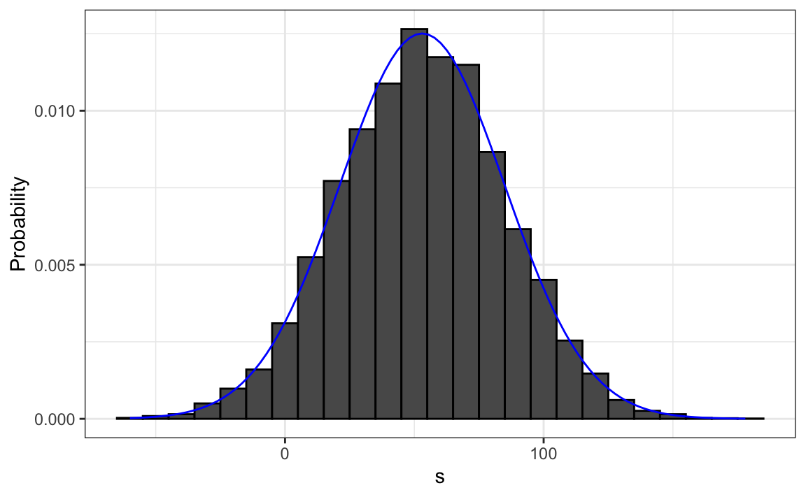
The probability distribution

We see that the distribution appears to be approximately normal.
A QQ-plot will confirm that the normal approximation is close to a perfect approximation.

The probability distribution

Remeber, if the distribution is normal, all we need to define it are the average and the standard deviation (SD).
Since we have the original values from which the distribution is created, we can easily compute these with mean(s) and sd(s).
The blue curve added to the histogram is a normal density with this average and standard deviation.

The probability distribution

This average and this standard deviation have special names; they are referred to as the expected value and standard error (SE) of the random variable $S$.

Note

Statistical theory offers a method to derive the distribution of random variables defined as the sum of independent random draw of numbers from an urn:
Specifically, in our example above, we can demonstrate that $(S+n)/2$ follows a binomial distribution.
We therefore do not need to run Monte Carlo simulations to determine the probability distribution of $S$.
The simulations were conducted for illustrative purposes.
We can use the function dbinom and pbinom to compute the probabilities exactly.

n <- 1000 
pbinom(n/2 - 1, size = n, prob = 10/19) 
#> [1] 0.0448

Distributions versus probability distributions

Before we continue, let’s establish an important distinction and connection between the distribution of a list of numbers and a probability distribution.
Any list of numbers $x_1,\dots,x_n$ has a distribution.
It does not have a probability distribution because they are not random.

Distributions versus probability distributions

We define $F(a)$ as the function that indicates what proportion of the list is less than or equal to $a$.
Given their usefulness as summaries when the distribution is approximately normal, we also define the average and standard deviation.

Distributions versus probability distributions

These are determined with a straightforward operation involving the vector containing the list of numbers, denoted as x:

m <- sum(x)/length(x) 
s <- sqrt(sum((x - m)^2)/length(x))

Distributions versus probability distributions

A random variable $X$ has a distribution function.
To define this, we do not need a list of numbers; it is a theoretical concept.
We define the distribution as the $F(a)$ that answers the question: What is the probability that $X$ is less than or equal to $a$?

Distributions versus probability distributions

However, if $X$ is defined by drawing from an urn containing numbers, then there is a list: the list of numbers inside the urn.
In this case, the distribution of that list is the probability distribution of $X$, and the average and standard deviation of that list are the expected value and standard error of the random variable.

Distributions versus probability distributions

Another way to think about it without involving an urn is by running a Monte Carlo simulation and generating a very large list of outcomes of $X$.

Distributions versus probability distributions

These outcomes form a list of numbers, and the distribution of this list will be a very good approximation of the probability distribution of $X$.
The longer the list, the better the approximation.
The average and standard deviation of this list will approximate the expected value and standard error of the random variable.

Notation for random variables

In statistical textbooks, upper case letters denote random variables, and we will adhere to this convention.
Lower case letters are used for observed values.
You will see some notation that include both.
For example, you will see events defined as $X \leq x$.
Here $X$ is a random variable and $x$ is an arbitrary value and not random.

Notation for random variables

So, for example, $X$ might represent the number on a die roll and $x$ will represent an actual value we see: 1, 2, 3, 4, 5, or 6.
In this case, the probability of $X=x$ is 1/6 regardless of the observed value $x$.
We can discuss what we expect $X$ to be, what values are probable, but we can’t discuss what value $X$ is.

Notation for random variables

Once we have data, we do see a realization of $X$.
Therefore, data analysts often speak of what could have been after observing what actually happened.

The expected value and SE

We will now review the mathematical theory that allows us to approximate the probability distributions for the sum of draws.
The same approach we use for the sum of draws will be useful for describing the distribution of averages and proportion, which we will need to understand how polls work.
The first important concept to learn is the expected value.

The expected value and SE

In statistics books, it is common to represent the expected value of the random variable $X$ with the letter $\mbox{E}$ like this:

\[\mbox{E}[X]\]

The expected value and SE

A random variable will vary around its expected value in a manner that if you take the average of many, many draws, the average will approximate the expected value.
This approximation improves as you take more draws, making the expected value a useful quantity to compute.

The expected value and SE

For discrete random variable with possible outcomes $x_1,\dots,x_n$, the expected value is defined as:

\[ \mbox{E}[X] = \sum_{i=1}^n x_i \,\mbox{Pr}(X = x_i) \]

The expected value and SE

Note that in the case that we are picking values from an urn, and each value $x_i$ has an equal chance $1/n$ of being selected, the above equation is simply the average of the $x_i$s.

\[ \mbox{E}[X] = \frac{1}{n}\sum_{i=1}^n x_i \]

The expected value and SE

If $X$ is a continuous random variable with a range of values $a$ to $b$ and a probability density function $f(x)$, this sum transforms into an integral:

\[ \mbox{E}[X] = \int_a^b x f(x) \]

The expected value and SE

In the urn used to model betting on red in roulette, we have 20 one-dollar bills and 18 negative one-dollar bills, so the expected value is:

\[ \mbox{E}[X] = (20 + -18)/38 \]

which is about 5 cents.

The expected value and SE

You might consider it a bit counterintuitive to say that $X$ varies around 0.05 when it only takes the values 1 and -1.
To make sense of the expected value in this context is by realizing that, if we play the game over and over, the casino wins, on average, 5 cents per game.

The expected value and SE

A Monte Carlo simulation confirms this:

B <- 10^6 
x <- sample(c(-1, 1), B, replace = TRUE, prob = c(9/19, 10/19)) 
mean(x) 
#> [1] 0.0522

The expected value and SE

In general, if the urn has two possible outcomes, say $a$ and $b$, with proportions $p$ and $1-p$ respectively, the average is:

\[\mbox{E}[X] = ap + b(1-p)\]

The expected value and SE

To confirm this, observe that if there are $n$ beads in the urn, then we have $np$ $a$s and $n(1-p)$ $b$s, and because the average is the sum, $n\times a \times p + n\times b \times (1-p)$, divided by the total $n$, we get that the average is $ap + b(1-p)$.

The expected value and SE

The reason we define the expected value is because this mathematical definition turns out to be useful for approximating the probability distributions of sum.
This, in turn, is useful for describing the distribution of averages and proportions.

The expected value and SE

The first useful fact is that the expected value of the sum of the draws is the number of draws $\times$ the average of the numbers in the urn.
Therefore, if 1,000 people play roulette, the casino expects to win, on average, about 1,000 $\times$ $0.05 = $50.

The expected value and SE

However, this is an expected value.
How different can one observation be from the expected value? The casino really needs to know this.
What is the range of possibilities? If negative numbers are too likely, they will not install roulette wheels.
Statistical theory once again answers this question.

The expected value and SE

The standard error (SE) gives us an idea of the size of the variation around the expected value.
In statistics books, it’s common to use:

\[\mbox{SE}[X] = \sqrt{\mbox{Var}[X]}\]

The expected value and SE

to denote the standard error of a random variable.
For discrete random variable with possible outcomes $x_1,\dots,x_n$, the standard error is defined as:

\[ \mbox{SE}[X] = \sqrt{\sum_{i=1}^n \left(x_i - E[X]\right)^2 \,\mbox{Pr}(X = x_i)}, \]

which you can think of as the expected average distance of $X$ from the expected value.

The expected value and SE

Note that in the case that we are picking values from an un urn where each value $x_i$ has an equal chance $1/n$ of being selected, the above equation is simply the standard deviation of of the $x_i$s.

\[ \mbox{SE}[X] = \sqrt{\frac{1}{n}\sum_{i=1}^n (x_i - \bar{x})^2} \mbox{ with } \bar{x} = \frac{1}{n}\sum_{i=1}^n x_i \]

The expected value and SE

If $X$ is a continuous random variable, with range of values $a$ to $b$ and probability density function $f(x)$, this sum turns into an integral:

\[ \mbox{SE}[X] = \sqrt{\int_a^b \left(x-\mbox{E}[X]\right)^2 f(x)\,\mathrm{d}x} \]

The expected value and SE

Using the definition of standard deviation, we can derive, with a bit of math, that if an urn contains two values $a$ and $b$ with proportions $p$ and $(1-p)$, respectively, the standard deviation is:

\[| b - a |\sqrt{p(1-p)}.\]

The expected value and SE

So in our roulette example, the standard deviation of the values inside the urn is:

\[ | 1 - (-1) | \sqrt{10/19 \times 9/19} \]

or:

2*sqrt(90)/19 
#> [1] 0.999

The expected value and SE

Since one draw is obviously the sum of just one draw, we can use the formula above to calculate that the random variable defined by one draw has an expected value of 0.05 and a SE of about 1.
This makes sense since we obtain either 1 or -1, with 1 slightly favored over -1.

The expected value and SE

A widely used mathematical result is that if our draws are independent, then the standard error of the sum is given by the equation:

\[ \sqrt{\mbox{number of draws}} \times \mbox{ SD of the numbers in the urn} \]

The expected value and SE

Using this formula, the sum of 1,000 people playing has standard error of about $32:

n <- 1000 
sqrt(n)*2*sqrt(90)/19 
#> [1] 31.6

The expected value and SE

As a result, when 1,000 people bet on red, the casino is expected to win $50 with a standard error of $32.
It therefore seems like a safe bet to install more roulette wheels.
But we still haven’t answered the question: How likely is the casino to lose money? The CLT will help in this regard.

Note

The exact probability for the casino winnings can be computed precisely, rather than approximately, using the binomial distribution.
However, here we focus on the CLT, which can be applied more broadly to sums of random variables in a way that the binomial distribution cannot.

Central Limit Theorem

The Central Limit Theorem (CLT) tells us that when the number of draws, also called the sample size, is large, the probability distribution of the sum of the independent draws is approximately normal.
Given that sampling models are used for so many data generation processes, the CLT is considered one of the most important mathematical insights in history.

Central Limit Theorem

Previously, we discussed that if we know that the distribution of a list of numbers is approximated by the normal distribution, all we need to describe the list are the average and standard deviation.
We also know that the same applies to probability distributions.

Central Limit Theorem

If a random variable has a probability distribution that is approximated with the normal distribution, then all we need to describe the probability distribution are the average and standard deviation, referred to as the expected value and standard error.

Central Limit Theorem

We previously ran this Monte Carlo simulation:

n <- 1000 
B <- 10000 
roulette_winnings <- function(n){ 
  x <- sample(c(-1, 1), n, replace = TRUE, prob = c(9/19, 10/19)) 
  sum(x) 
} 
s <- replicate(B, roulette_winnings(n))

Central Limit Theorem

The Central Limit Theorem (CLT) tells us that the sum $S$ is approximated by a normal distribution.
Using the formulas above, we know that the expected value and standard error are:

n * (20 - 18)/38  
#> [1] 52.6
sqrt(n)*2*sqrt(90)/19  
#> [1] 31.6

Central Limit Theorem

The theoretical values above match those obtained with the Monte Carlo simulation:

mean(s) 
#> [1] 52.6
sd(s) 
#> [1] 31.5

Central Limit Theorem

Using the CLT, we can skip the Monte Carlo simulation and instead compute the probability of the casino losing money using this approximation:

mu <- n*(20 - 18)/38 
se <- sqrt(n)*2*sqrt(90)/19  
pnorm(0, mu, se) 
#> [1] 0.0478

which is also in very good agreement with our Monte Carlo result:

mean(s < 0) 
#> [1] 0.0442

How large is large in the CLT?

The CLT works when the number of draws is large, but “large” is a relative term.
In many circumstances, as few as 30 draws is enough to make the CLT useful.
In some specific instances, as few as 10 is enough.
However, these should not be considered general rules.
Note that when the probability of success is very small, much larger sample sizes are needed.

How large is large in the CLT?

By way of illustration, let’s consider the lottery.
In the lottery, the chances of winning are less than 1 in a million.
Thousands of people play so the number of draws is very large.
Yet the number of winners, the sum of the draws, range between 0 and 4.
This sum is certainly not well approximated by a normal distribution, so the CLT does not apply, even with the very large sample size.

How large is large in the CLT?

This is generally true when the probability of a success is very low.
In these cases, the Poisson distribution is more appropriate.
You can explore the properties of the Poisson distribution using dpois and ppois.
You can generate random variables following this distribution with rpois.
However, we won’t cover the theory here.

How large is large in the CLT?

You can learn about the Poisson distribution in any probability textbook and even Wikipedia

Statistical properties of averages

There are several useful mathematical results that we used above and often employ when working with data.
We list them below.

Property 1

The expected value of the sum of random variables is the sum of each random variable’s expected value.
We can write it like this:

\[ \mbox{E}[X_1+X_2+\dots+X_n] = \mbox{E}[X_1] + \mbox{E}[X_2]+\dots+\mbox{E}[X_n] \]

Property 1

If $X$ represents independent draws from the urn, then they all have the same expected value.
Let’s denote the expected value with $\mu$ and rewrite the equation as:

\[ \mbox{E}[X_1+X_2+\dots+X_n]= n\mu \]

which is another way of writing the result we show above for the sum of draws.

Property 2

The expected value of a non-random constant times a random variable is the non-random constant times the expected value of a random variable.
This is easier to explain with symbols:

\[ \mbox{E}[aX] = a\times\mbox{E}[X] \]

Property 2

To understand why this is intuitive, consider changing units.
If we change the units of a random variable, such as from dollars to cents, the expectation should change in the same way.

Property 2

A consequence of the above two facts is that the expected value of the average of independent draws from the same urn is the expected value of the urn, denoted as $\mu$ again:

\[ \mbox{E}[(X_1+X_2+\dots+X_n) / n]= \mbox{E}[X_1+X_2+\dots+X_n] / n = n\mu/n = \mu \]

Property 3

The square of the standard error of the sum of independent random variables is the sum of the square of the standard error of each random variable.
This one is easier to understand in math form:

\[ \mbox{SE}[X_1+X_2+\dots+X_n] = \sqrt{\mbox{SE}[X_1]^2 + \mbox{SE}[X_2]^2+\dots+\mbox{SE}[X_n]^2 } \]

Property 3

The square of the standard error is referred to as the variance in statistical textbooks.
Note that this particular property is not as intuitive as the previous three and more in depth explanations can be found in statistics textbooks.

Property 4

The standard error of a non-random constant times a random variable is the non-random constant times the random variable’s standard error.
As with the expectation:

\[ \mbox{SE}[aX] = a \times \mbox{SE}[X] \]

To see why this is intuitive, again think of units.

Property 4

A consequence of 3 and 4 is that the standard error of the average of independent draws from the same urn is the standard deviation of the urn divided by the square root of $n$ (the number of draws), call it $\sigma$:

\[ \begin{aligned} \mbox{SE}[(X_1+X_2+\dots+X_n) / n] &= \mbox{SE}[X_1+X_2+\dots+X_n]/n \\ &= \sqrt{\mbox{SE}[X_1]^2+\mbox{SE}[X_2]^2+\dots+\mbox{SE}[X_n]^2}/n \\ &= \sqrt{\sigma^2+\sigma^2+\dots+\sigma^2}/n\\ &= \sqrt{n\sigma^2}/n\\ &= \sigma / \sqrt{n} \end{aligned} \]

Property 5

If $X$ is a normally distributed random variable, then if $a$ and $b$ are non-random constants, $aX + b$ is also a normally distributed random variable.
All we are doing is changing the units of the random variable by multiplying by $a$, then shifting the center by $b$.

Notation

Note that statistical textbooks use the Greek letters $\mu$ and $\sigma$ to denote the expected value and standard error, respectively.
This is because $\mu$ is the Greek letter for $m$, the first letter of mean, which is another term used for expected value.
Similarly, $\sigma$ is the Greek letter for $s$, the first letter of standard error.

The assumption of independence is important

The given equation reveals crucial insights for practical scenarios.
Specifically, it suggests that the standard error can be minimized by increasing the sample size, $n$, and we can quantify this reduction.
However, this principle holds true only when the variables $X_1, X_2, \dots, X_n$ are independent.
If they are not, the estimated standard error can be significantly off.

The assumption of independence is important

We later introduce the concept of correlation, which quantifies the degree to which variables are interdependent.
If the correlation coefficient among the $X$ variables is $\rho$, the standard error of their average is:

\[ \mbox{SE}\left(\bar{X}\right) = \sigma \sqrt{\frac{1 + (n-1) \rho}{n}} \]

The assumption of independence is important

The key observation here is that as $\rho$ approaches its upper limit of 1, the standard error increases.
Notably, in the situation where $\rho = 1$, the standard error, $\mbox{SE}(\bar{X})$, equals $\sigma$, and it becomes unaffected by the sample size $n$.

Law of large numbers

An important implication of result 4 above is that the standard error of the average becomes smaller and smaller as $n$ grows larger.
When $n$ is very large, then the standard error is practically 0 and the average of the draws converges to the average of the urn.
This is known in statistical textbooks as the law of large numbers or the law of averages.

Misinterpretation of the law of averages

The law of averages is sometimes misinterpreted.
For example, if you toss a coin 5 times and see a head each time, you might hear someone argue that the next toss is probably a tail because of the law of averages: on average we should see 50% heads and 50% tails.

Misinterpretation of the law of averages

A similar argument would be to say that red “is due” on the roulette wheel after seeing black come up five times in a row.
Yet these events are independent so the chance of a coin landing heads is 50%, regardless of the previous 5.

Misinterpretation of the law of averages

The same principle applies to the roulette outcome.
The law of averages applies only when the number of draws is very large and not in small samples.

Misinterpretation of the law of averages

After a million tosses, you will definitely see about 50% heads regardless of the outcome of the first five tosses.
Another funny misuse of the law of averages is in sports when TV sportscasters predict a player is about to succeed because they have failed a few times in a row.