Introduction to Probability

2024-10-21

Probability

• The term probability is used in everyday language.

• Yet answering questions about probability is often hard, if not impossible.

• In contrast probability has a very intuitive definition in games of chance.

• Today we discuss a mathematical definition of probability that allows us to give precise answers to certain questions.

Probability

• Probability Theory was born because certain mathematcial computations can give an advantage in games of chance.

• Probability continues to be highly useful in modern games of chance.

• Probability theory is also useful whenever our data is affected by chance in some manner.

• A knowledge of probability is indispensable for addressing most data analysis challenges.

Probability

• In today’s lecture, we will use casino games to illustrate the fundamental concepts.

• Instead of diving into the mathematical theories, we will uses R to demonstrate these concepts.

• Understanding the connection between probability theory and real world data analysis is a bit more challenging. We will be discussing this connection throughout the rest of the course.

Definitions and Notation

• Events are fundamental concepts that help us understand and quantify uncertainty in various situations.

• An event is defined as a specific outcome or a collection of outcomes from a random experiment.

Definitions and Notation

• Simple examples of events can be constructed with urns.

• If we have 2 red beads and 3 blue beads inside an urn, and we perform the random experiment of picking 1 bead, there are two outcomes: bead is red or blue.

beads <- rep( c("red", "blue"), times = c(2,3))

• The four possible events: bead is red, bead is blue, bead is red or blue, and an event with no outcomes.

Definitions and Notation

• In more complex random experiment, we can define many more events.

• For example if the random experiment is picking 2 beads, we can define events such as first bead is red, second bead is blue, both beads are red, and so on.

• In a random experiment such as political poll, where we randomly phone 100 likely voters at random, we can form many million events, for example calling 48 Democrats and 52 Republicans.

Definitions and Notation

• We usually use capital letters \(A\), \(B\), \(C\), … to to denote events.

• If we denote an event as \(A\) then we use the notation \(\mbox{Pr}(A)\) to denote the probability of event \(A\) occurring.

Definitions and Notation

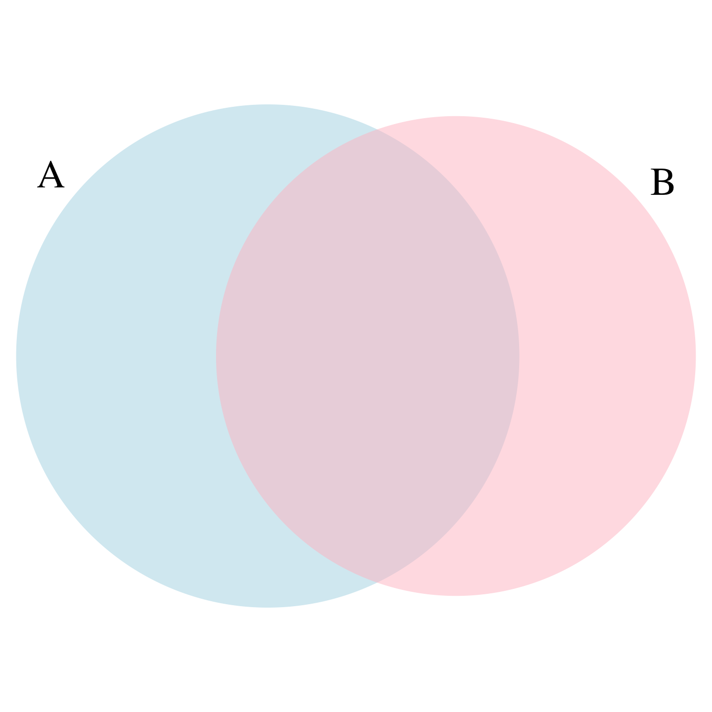
• We can combine events in different ways to form new events. For example, if event

• \(A\)=first bead is red and second bead is blue, and

• \(B\)=first bead is red and second bead is red

• then \(A \cup B\) (\(A\) or \(B\)) is the event first bead is red,

• while \(A \cap B\) (\(A\) and \(B\)) is the empty event since both can’t happen.

Definitions and Notation

• With continuous variables, events will relate to questions, such as Is this person taller than 6 feet?

• In these cases, we represent events in a more mathematical form: \(A = X > 6\).

Independence

• Many examples of events that are not independent come from card games.

• When we deal the first card, the probability of getting a King is 1/13 since there are thirteen possibilities: Ace, Deuce, Three, \(\dots\), Ten, Jack, Queen, King, and Ace.

• If we deal a King for the first card, the probability of a second card being a King decreases because there are only three Kings left: The probability is 3 out of 51.

Independence

• By detault, the sample function samples without replacement

set.seed(1996)
x <- sample(beads, 5) 

• If you have to guess the color of the first bead, you will predict blue since blue has a 60% chance.

Independence

• However, if I show you the result of the last four outcomes:

x[2:5] 

[1] "blue" "blue" "red"  "blue"

• would you still guess blue? Of course not.

Conditional probabilities

• When events are not independent, conditional probabilities are useful.

• We use the \(|\) to shorten conditional on. For example:

\[ \mbox{Pr}(\mbox{Card 2 is a king} \mid \mbox{Card 1 is a king}) = 3/51 \]

Conditional probabilities

• When two events, say \(A\) and \(B\), are independent, we have:

\[ \mbox{Pr}(A \mid B) = \mbox{Pr}(A) \]

• In fact, this can be considered the mathematical definition of independence.

Multiplication rule

• If we want to determine the probability of two events, say \(A\) and \(B\), occurring, we can use the multiplication rule:

\[ \mbox{Pr}(A \cup B) = \mbox{Pr}(A)\mbox{Pr}(B \mid A) \]

Multiplication rule

• For example:

\[ \mbox{Pr}(\mbox{Blackjack in first hand}) = \\ \mbox{Pr}(\mbox{Ace first})\mbox{Pr}(\mbox{Face card second}\mid \mbox{Ace first}) +\\ \mbox{Pr}(\mbox{Face card first})\mbox{Pr}(\mbox{Ace}\mid \mbox{Face card second}) =\\ \frac{1}{13}\frac{16}{51} + \frac{4}{13}\frac{4}{51} \approx 0.0483 \]

Multiplication rule

• We can use induction to expand for more events:

\[ \mbox{Pr}(A \cup B \cup C) = \mbox{Pr}(A)\mbox{Pr}(B \mid A)\mbox{Pr}(C \mid A \cup B) \]

Multiplication rule

• When dealing with independent events, the multiplication rule becomes simpler:

\[ \mbox{Pr}(A \cup B \cup C) = \mbox{Pr}(A)\mbox{Pr}(B)\mbox{Pr}(C) \]

• However, we have to be very careful before using this version of the multiplication rule, since assuming independence can result in very different and incorrect probability calculations when events are not actually independent.

Multiplication rule example

• Imagine a court case in which the suspect was described as having a mustache and a beard.

• The defendant has both and an “expert” testifies that 1/10 men have beards and 1/5 have mustaches.

• Using the multiplication rule, he concludes that \(1/10 \times 1/5\) or 0.02 have both.

• But this assumes independence!

• If the conditional probability of a man having a mustache, conditional on him having a beard, is .95, then the probability is: \(1/10 \times 95/100 = 0.095\)

Multiplication rule under

• The multiplication rule also gives us a general formula for computing conditional probabilities:

\[ \mbox{Pr}(B \mid A) = \frac{\mbox{Pr}(A \cup B)}{ \mbox{Pr}(A)} \]

Addition rule

• The addition rule tells us that:

\[ \mbox{Pr}(A \cap B) = \mbox{Pr}(A) + \mbox{Pr}(B) - \mbox{Pr}(A \cup B) \]

Random Variables

• Random variables are numeric outcomes resulting from random processes.

• We can easily generate random variables using the simple examples we have shown.

• For example, define X to be 1 if a bead is blue and red otherwise:

beads <- rep( c("red", "blue"), times = c(2,3))
x <- ifelse(sample(beads, 1) == "blue", 1, 0)

Random Variables

• Here X is a random variable, changing randomly each time we select a new bead. Sometimes it’s 1 and sometimes it’s 0.

ifelse(sample(beads, 1) == "blue", 1, 0)

[1] 0

ifelse(sample(beads, 1) == "blue", 1, 0)

[1] 1

ifelse(sample(beads, 1) == "blue", 1, 0)

[1] 0

Random Variables

• More interesting random variables are:
  • the number of times we win in a game of chance,
  • the number of democrats in a random sample of 1,000 voters, and
  • the proportion of patients randomly assigned to a control group in drug trial.

Discrete probability

If I have 2 red beads and 3 blue beads inside an urn and I pick one at random, what is the probability of picking a red one? Our intuition tells us that the answer is 2/5 or 40%.

Discrete probability

• A precise definition can be given by noting that there are five possible outcomes, of which two satisfy the condition necessary for the event pick a red bead.

• Since each of the five outcomes has an equal chance of occurring, we conclude that the probability is .4 for red and .6 for blue.

Discrete probability

• A more tangible way to think about the probability of an event is as the proportion of times the event occurs when we repeat the experiment an infinite number of times, independently, and under the same conditions.

• This is the frequentist way of thinking about probability.

Monte Carlo

• Monte Carlo simulations use computers to perform these experiments.

• Random number generators permit us to mimic the process of picking at random.

• The sample function in R uses a random number generator:

beads <- rep(c("red", "blue"), times = c(2,3))
sample(beads, 1)

[1] "blue"

Monte Carlo

• If we repeat the experiment over and over, we can define the probability using the frequentists definition

n <- 10^7
x <- sample(beads, n, replace = TRUE)
table(x)/n

x
     blue       red 
0.6002232 0.3997768 

• Note the definition is for \(n=\infty\). In practice we use very large numbers tp get very close.

Probability distributions

An example of a probability distribution is:

Pr(picking a Republican)	=	0.44
Pr(picking a Democrat)	=	0.44
Pr(picking an undecided)	=	0.10
Pr(picking a Green)	=	0.02

Setting the random seed

• Before we continue, we will briefly explain the function set.seed

set.seed(2020-10-13)  

• When using random number generators you get a different answer each time.

• This is fine, but if you want to ensure that results are consistent with each run, you can set R’s random number generation seed to a specific number.

Combinations and permutations

• Being able to count combinations and permutations is an important part of performing discrete probability computations.

• We will not cover this but you should know the function expand.grid

• and the gtools functions permutatios and combinations.

Combinations and permutations

• Here is how we generate a deck of cards:

suits <- c("Diamonds", "Clubs", "Hearts", "Spades") 
numbers <- c("Ace", "Deuce", "Three", "Four", "Five", "Six", "Seven",  
             "Eight", "Nine", "Ten", "Jack", "Queen", "King") 
deck <- expand.grid(number = numbers, suit = suits) 
deck <- paste(deck$number, deck$suit) 

Combinations and permutations

• Here are all the ways we can choose two numbers from a list consisting of 1,2,3:

library(gtools) 
permutations(3, 2) 

     [,1] [,2]
[1,]    1    2
[2,]    1    3
[3,]    2    1
[4,]    2    3
[5,]    3    1
[6,]    3    2

• The order matters here: 3,1 is different than 1,3.

• (1,1), (2,2), and (3,3) do not appear because once we pick a number, it can’t appear again.

Combinations and permutations

• To compute all possible ways we can choose two cards when the order matters, we type, you can use the v option:

hands <- permutations(52, 2, v = deck) 

Combinations and permutations

• What about if the order does not matter? For example, in Blackjack, if you obtain an Ace and a face card in the first draw, it is called a Natural 21, and you win automatically.

• If we wanted to compute the probability of this happening, we would enumerate the combinations, not the permutations, since the order does not matter.

combinations(3,2) 

     [,1] [,2]
[1,]    1    2
[2,]    1    3
[3,]    2    3

Infinity in practice

• The theory described here requires repeating experiments over and over indefinitely.

• In practice, we can’t do this.

• In the problem set you will be asked to explore how we implement asymptotic theory in practice.

Continuous probability

• When summarizing a list of numeric values, such as heights, it is not useful to construct a distribution that defines a proportion to each possible outcome.

• Similarly, for a random variable that can take any value in a continuous set, it impossible to assign a positive probabilities to the infinite number of possible values.

• Here, we outline the mathematical definitions of distributions for continuous random variables and useful approximations frequently employed in data analysis.

CDF

• We used the heights of adult male students as an example:

library(tidyverse) 
library(dslabs) 
x <- heights %>% filter(sex == "Male") %>% pull(height) 

• and defined the empirical cumulative distribution function (eCDF) as.

F <- function(a) mean(x <= a) 

• which, for any value a, gives the proportion of values in the list x that are smaller or equal than a.

CDF

• There is a connection to the empirical CDF.

• If I randomly pick one of the male students, what is the chance that he is taller than 70.5 inches?

• Since every student has the same chance of being picked, the answer is the proportion of students that are taller than 70.5 inches.

CDF

• Using the eCDF we obtain an answer by typing:

1 - F(70) 

[1] 0.3768473

• The CDF is a version of the eCDF that assigns theoretical probabilities for each \(a\) rather than proportions computed from data.

CDF

• Although, as we just demonstrated, proportions computed from data can be used to define probabilities for a random variable.

• Specifically, the CDF for a random outcome \(X\) defines, for any number \(a\), the probability of observing a value larger than \(a\).

\[ F(a) = \mbox{Pr}(X \leq a) \]

• Once a CDF is defined, we can use it to compute the probability of any subset of values.

CDF

• For instance, the probability of a student being between height a and height b is:

\[ \mbox{Pr}(a < X \leq b) = F(b)-F(a) \]

• Since we can compute the probability for any possible event using this approach, the CDF defines the probability distribution.

Probability density function

• A mathematical result that is very useful in practice is that, for most CDFs, we can define a function, call it \(f(x)\), that permits us to construct the CDF using Calculus, like this:

\[ F(b) - F(a) = \int_a^b f(x)\,dx \]

• \(f(x)\) is referred to as the probability density function.

Probability density function

• The intuition is that even for continuous outcomes we can define tiny intervals, that are almost as small as points, that have positive probabilities.

• If we think of the size of these intervals as the base of a rectangle, the probability density function \(f\) determines the height of the rectangle so that the summing up of the area of these rectangles approximate the probability \(F(b) - F(a)\).

Probability density function

• This sum can be written as Reimann sum that is approximated by an integral:

Probability density function

• An example of such a continuous distribution is the normal distribution.

• The probability density function is given by:

\[f(x) = e^{-\frac{1}{2}\left( \frac{x-m}{s} \right)^2} \]

• The cumulative distribution for the normal distribution is defined by a mathematical formula which in R can be obtained with the function pnorm.

Probability density function

• We say that a random quantity is normally distributed with average m and standard deviation s if its probability distribution is defined by:

F(a) = pnorm(a, m, s) 

Probability density function

• This is useful because, if we are willing to use the normal approximation we don’t need the entire dataset to answer questions such as: What is the probability that a randomly selected student is taller then 70 inches?

• We just need the average height and standard deviation:

m <- mean(x) 
s <- sd(x) 
1 - pnorm(70.5, m, s) 

[1] 0.371369

Distributions as approximations

• The normal distribution is derived mathematically; we do not need data to define it.

• For practicing data scientists, almost everything we do involves data.

• Data is always, technically speaking, discrete.

• For example, we could consider our height data categorical, with each specific height a unique category.

• The probability distribution is defined by the proportion of students reporting each height.

Distributions as approximations

• Below is a plot of that probability distribution:

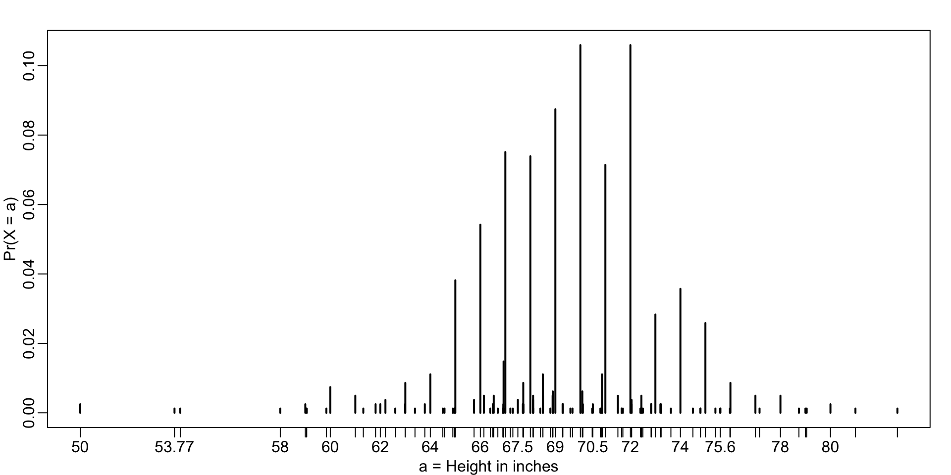
Distributions as approximations

• While most students rounded up their heights to the nearest inch, others reported values with more precision.

• One student reported his height to be 69.6850393700787, which is 177 centimeters.

• The probability assigned to this height is 0.0012315 or 1 in 812.

Distributions as approximations

• The probability for 70 inches is much higher at 0.1059113,

• Does it really make sense to think of the probability of being exactly 70 inches as being different than 69.6850393700787?

Distributions as approximations

• Clearly it is much more useful for data analytic purposes to treat this outcome as a continuous numeric variable, keeping in mind that very few people, or perhaps none, are exactly 70 inches, and that the reason we get more values at 70 is because people round to the nearest inch.

Distributions as approximations

• With continuous distributions, the probability of a singular value is not even defined.

• For instance, it does not make sense to ask what is the probability that a normally distributed value is 70.

• Instead, we define probabilities for intervals.

Distributions as approximations

• We therefore could ask, what is the probability that someone is between 69.5 and 70.5?

• In cases like height, in which the data is rounded, the normal approximation is particularly useful if we deal with intervals that include exactly one round number.

Distributions as approximations

• For example, the normal distribution is useful for approximating the proportion of students reporting values in intervals like the following three:

mean(x <= 68.5) - mean(x <= 67.5) 

[1] 0.114532

mean(x <= 69.5) - mean(x <= 68.5) 

[1] 0.1194581

mean(x <= 70.5) - mean(x <= 69.5) 

[1] 0.1219212

Distributions as approximations

• Note how close we get with the normal approximation:

pnorm(68.5, m, s) - pnorm(67.5, m, s)  

[1] 0.1031077

pnorm(69.5, m, s) - pnorm(68.5, m, s)  

[1] 0.1097121

pnorm(70.5, m, s) - pnorm(69.5, m, s)  

[1] 0.1081743

• However, the approximation is not as useful for other intervals.

Distributions as approximations

• For instance, notice how the approximation breaks down when we try to estimate:

mean(x <= 70.9) - mean(x <= 70.1) 

[1] 0.02216749

• with:

pnorm(70.9, m, s) - pnorm(70.1, m, s) 

[1] 0.08359562

Distributions as approximations

• In general, we call this situation discretization.

• Although the true height distribution is continuous, the reported heights tend to be more common at discrete values, in this case, due to rounding.

• As long as we are aware of how to deal with this reality, the normal approximation can still be a very useful tool.

The probability density

• For categorical distributions, we can define the probability of a category.

• For example, a roll of a die, let’s call it \(X\), can be 1, 2, 3, 4, 5 or 6.

• The probability of 4 is defined as:

\[ \mbox{Pr}(X=4) = 1/6 \]

The probability density

• The CDF can then easily be defined:

\[ F(4) = \mbox{Pr}(X\leq 4) = \mbox{Pr}(X = 4) + \mbox{Pr}(X = 3) + \mbox{Pr}(X = 2) + \mbox{Pr}(X = 1) \]

The probability density

• Although for continuous distributions the probability of a single value \(\mbox{Pr}(X=x)\) is not defined, there is a theoretical definition that has a similar interpretation.

• The probability density at \(x\) is defined as the function \(f(a)\) such that:

\[ F(a) = \mbox{Pr}(X\leq a) = \int_{-\infty}^a f(x)\, dx \]

The probability density

• For those that know calculus, remember that the integral is related to a sum: it is the sum of bars with widths approximating 0.

• If you don’t know calculus, you can think of \(f(x)\) as a curve for which the area under that curve, up to the value \(a\), gives you the probability \(\mbox{Pr}(X\leq a)\).

The probability density

• For example, to use the normal approximation to estimate the probability of someone being taller than 76 inches, we use:

1 - pnorm(76, m, s) 

[1] 0.03206008

The probability density

• which mathematically is the grey area:

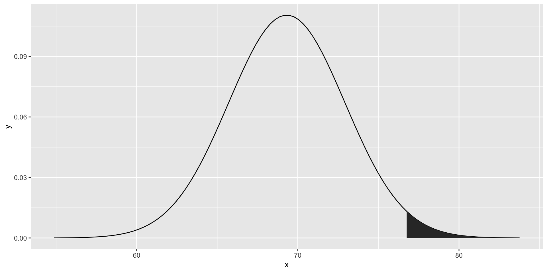
The probability density

• The curve you see is the probability density for the normal distribution.

• In R, we get this using the function dnorm.

• While it may not be immediately apparent why knowing about probability densities is useful, understanding this concept is essential for individuals aiming to fit models to data for which predefined functions are not available.

Monte Carlo

• R provides functions to generate normally distributed outcomes.

• Specifically, the rnorm function takes three arguments: size, average (defaults to 0), and standard deviation (defaults to 1), and produces random numbers.

Monte Carlo

• Here is an example of how we could generate data that looks like our reported heights:

n <- length(x) 
m <- mean(x) 
s <- sd(x) 
simulated_heights <- rnorm(n, m, s) 

Monte Carlo

• Not surprisingly, the distribution looks normal:

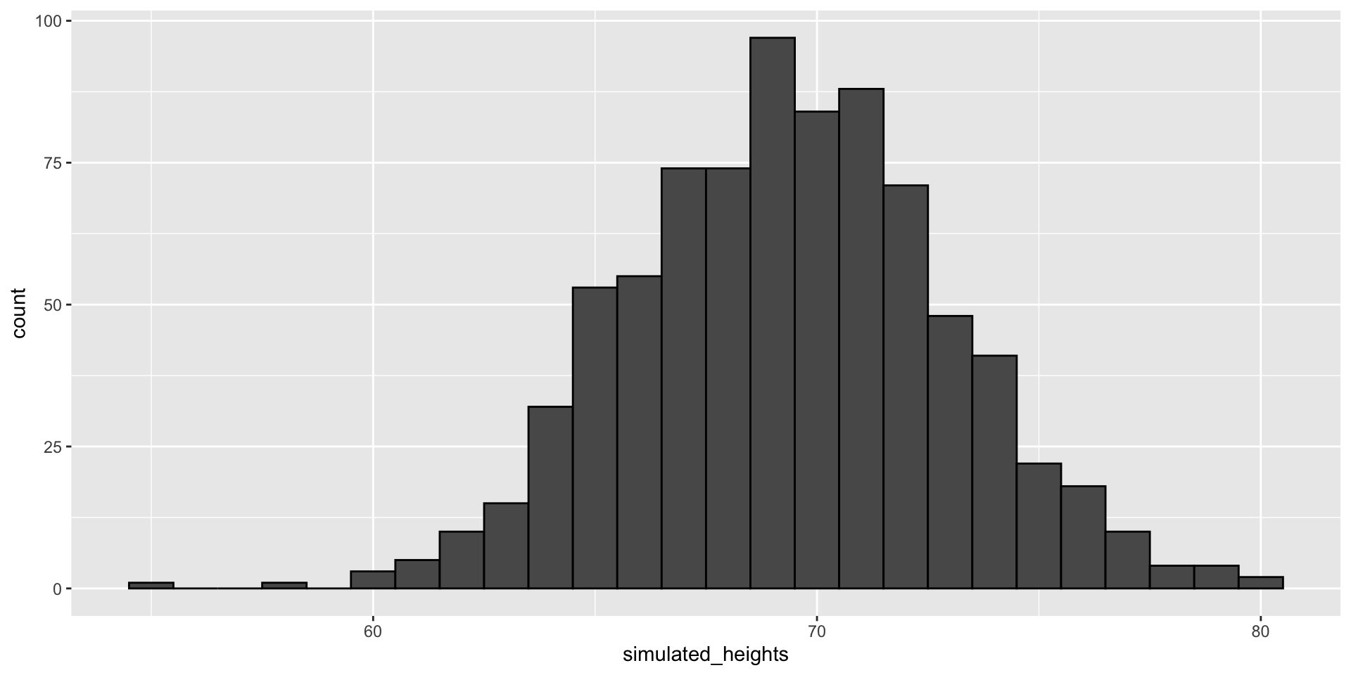
Monte Carlo

• This is one of the most useful functions in R, as it will permit us to generate data that mimics natural events and answers questions related to what could happen by chance by running Monte Carlo simulations.

• If, for example, we pick 800 males at random, what is the distribution of the tallest person? How rare is a seven-footer in a group of 800 males? The following Monte Carlo simulation helps us answer that question:

Monte Carlo

B <- 10000 
tallest <- replicate(B, { 
  simulated_data <- rnorm(800, m, s) 
  max(simulated_data) 
}) 

Monte Carlo

• Having a seven-footer is quite rare:

mean(tallest >= 7*12) 

[1] 0.0195

Monte Carlo

• Here is the resulting distribution:

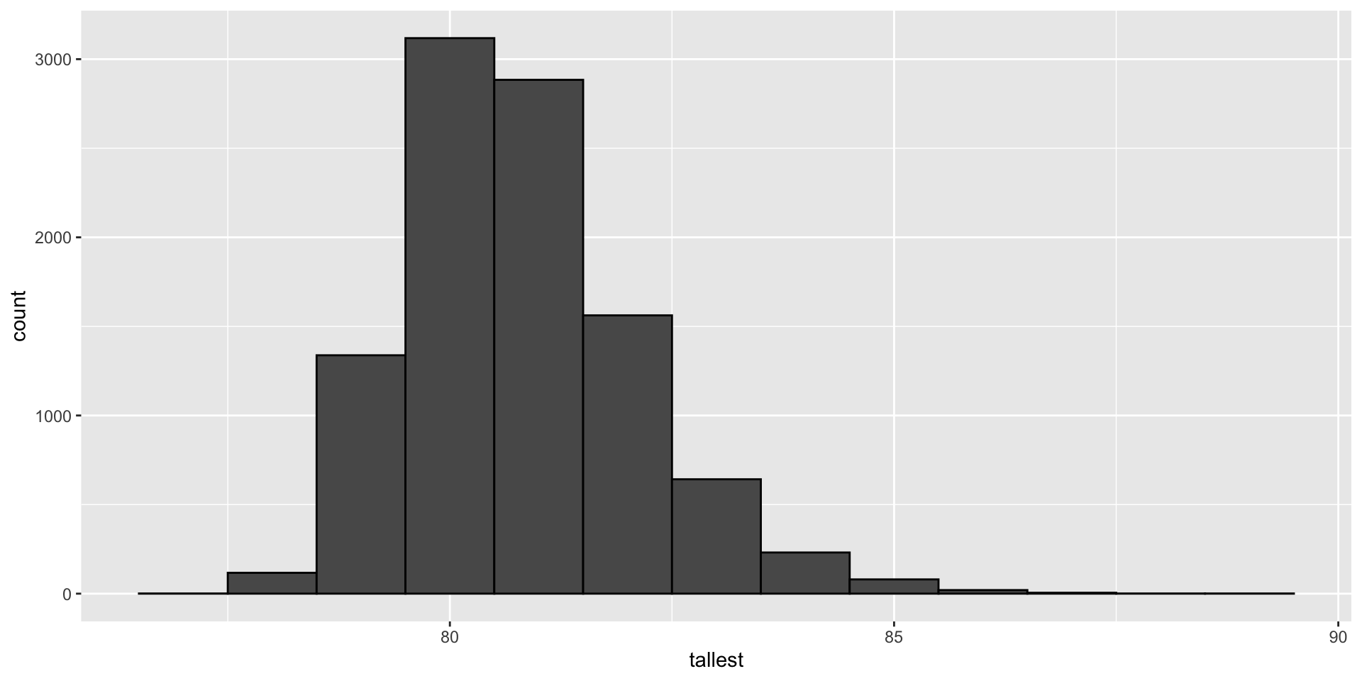
• Note that it does not look normal.

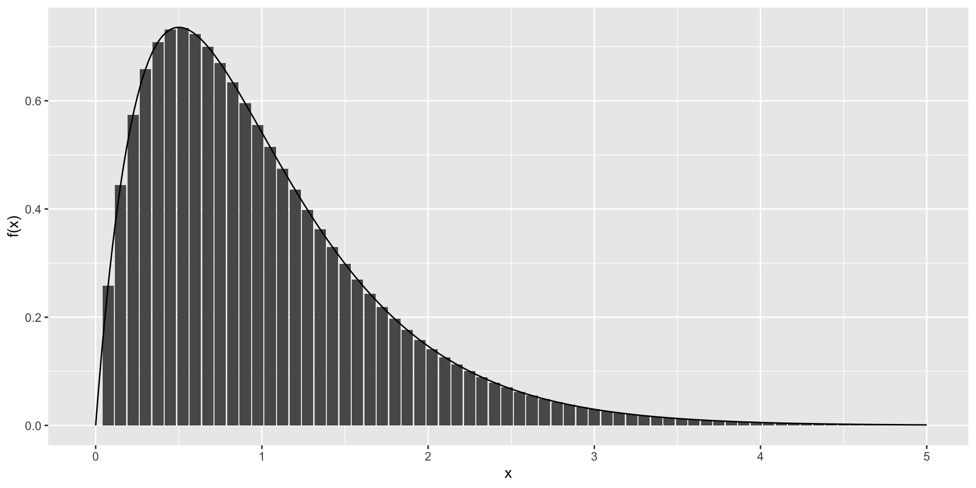
Continuous distributions

• The normal distribution is not the only useful theoretical distribution.

• Other continuous distributions that we may encounter are the student-t, Chi-square, exponential, gamma, beta, and beta-binomial.

• R provides functions to compute the density, the quantiles, the cumulative distribution functions and to generate Monte Carlo simulations.

• R uses a convention that lets us remember the names, namely using the letters d, q, p, and r in front of a shorthand for the distribution.

Continuous distributions

• We have already seen the functions dnorm, pnorm, and rnorm for the normal distribution.

• The functions qnorm gives us the quantiles.

• We can therefore draw a distribution like this:

Continuous distributions

x <- seq(-4, 4, length.out = 100) 
qplot(x, f, geom = "line", data = data.frame(x, f = dnorm(x)))