The caret package

2024-12-09

The caret package

There dozens of machine learning algorithms.
Many of these algorithms are implemented in R.
However, they are distributed via different packages, developed by different authors, and often use different syntax.
The caret package tries to consolidate these differences and provide consistency.

The caret package

It currently includes over 200 different methods which are summarized in the caret package manual.

The caret package

We use the 2 or 7 example to illustrate.
Then we apply it to the larger MNIST dataset.

The `train` function

Functions such as lm, glm, qda, lda, knn3, rpart and randomForrest use different syntax, have different argument names, and produce objects of different types.
The caret train function lets us train different algorithms using similar syntax.

The `train` function

For example, we can type the following to train three different models:

library(dslabs)
library(caret) 
train_glm <- train(y ~ ., method = "glm", data = mnist_27$train) 
train_qda <- train(y ~ ., method = "qda", data = mnist_27$train) 
train_knn <- train(y ~ ., method = "knn", data = mnist_27$train)

The `predict` function

The predict function is very useful for machine learning applications.
Here is an example with regression:

fit <- lm(y ~ ., data = mnist_27$train) 
p_hat <- predict(fit, newdata = mnist_27$test)

The `predict` function

In this case, the function is simply computing.

\[ \widehat{p}(\mathbf{x}) = \widehat{\beta}_0 + \widehat{\beta}_1 x_1 + \widehat{\beta}_2 x_2 \]

for the x_1 and x_2 in the test set mnist_27$test.

The `predict` function

With these estimates in place, we can make our predictions and compute our accuracy:

y_hat <- factor(ifelse(p_hat > 0.5, 7, 2))

The `predict` function

predict does not always return objects of the same type
it depends on what type of object it is applied to.
To learn about the specifics, you need to look at the help file specific for the type of fit object that is being used.

The `predict` function

predict is actually a special type of function in R called a generic function.
Generic functions call other functions depending on what kind of object it receives.
So if predict receives an object coming out of the lm function, it will call predict.lm.
If it receives an object coming out of glm, it calls predict.glm.
If from knn3, it calls predict.knn3, and so on.

The `predict` function

These functions are similar but not exactly.

?predict.glm 
?predict.qda 
?predict.knn3

There are many other versions of predict and many machine learning algorithms define their own predict function.

The `predict` function

As with train, caret unifies the use of predict with the function predict.train.
This function takes the output of train and produces prediction of categories or estimates of $p(\mathbf{x})$.

The `predict` function

The code looks the same for all methods:

y_hat_glm <- predict(train_glm, mnist_27$test, type = "raw") 
y_hat_qda <- predict(train_qda, mnist_27$test, type = "raw") 
y_hat_knn <- predict(train_knn, mnist_27$test, type = "raw")

This permits us to quickly compare the algorithms.

The `predict` function

For example, we can compare the accuracy like this:

fits <- list(glm = y_hat_glm, qda = y_hat_qda, knn = y_hat_knn) 
sapply(fits, function(fit){
  confusionMatrix(fit, mnist_27$test$y)$overall[["Accuracy"]]
})

  glm   qda   knn 
0.775 0.815 0.835

Resampling

When an algorithm includes a tuning parameter, train automatically uses a resampling method to estimate MSE and decide among a few default candidate values.
To find out what parameter or parameters are optimized, you can read the caret manual.

The `predict` function

Or study the output of:

modelLookup("knn")

To obtain all the details of how caret implements kNN you can use:

getModelInfo("knn")

Resampling

If we run it with default values:

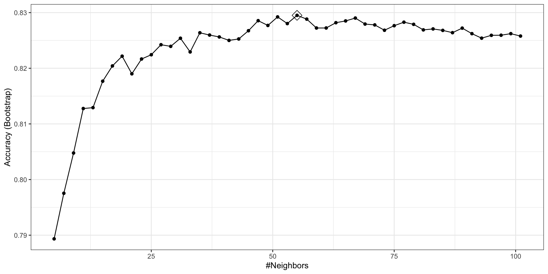
train_knn <- train(y ~ ., method = "knn", data = mnist_27$train)

you can quickly see the results of the cross validation using the ggplot function.

Resampling

ggplot(train_knn, highlight = TRUE)

The argument highlight highlights the max.

Resampling

By default, the resampling is performed by taking 25 bootstrap samples, each comprised of 25% of the observations.
We change this using the trControl argument. More on this later.
For the kNN method, the default is to try $k=5,7,9$.
We change this using the tuneGrid argument.

Resampling

Let’s try seq(5, 101, 2).
Since we are fitting $49 \times 25 = 1225$ kNN models, running this code will take several seconds.

set.seed(2003)
train_knn <- train(y ~ ., method = "knn",  
                   data = mnist_27$train, 
                   tuneGrid = data.frame(k = seq(5, 101, 2)))

Resampling

ggplot(train_knn, highlight = TRUE)

Note

Because resampling methods are random procedures, the same code can result in different results.
To assure reproducible results you should set the seed, as we did at the start of this chapter.

Resampling

To access the parameter that maximized the accuracy, you can use this:

train_knn$bestTune

    k
26 55

and the best performing model like this:

train_knn$finalModel

55-nearest neighbor model
Training set outcome distribution:

  2   7 
401 399

Resampling

The function predict will use this best performing model.
Here is the accuracy of the best model when applied to the test set, which we have not yet used because the cross validation was done on the training set:

confusionMatrix(predict(train_knn, mnist_27$test, type = "raw"), 
                mnist_27$test$y)$overall["Accuracy"]

Accuracy 
   0.825

Resampling

Bootstrapping is not always the best approach to resampling.
If we want to change our resampling method, we can use the trainControl function.
For example, the code below runs 10-fold cross validation.

Resampling

We accomplish this using the following code:

control <- trainControl(method = "cv", number = 10, p = .9) 
train_knn_cv <- train(y ~ ., method = "knn",  
                   data = mnist_27$train, 
                   tuneGrid = data.frame(k = seq(1, 71, 2)), 
                   trControl = control)

Note

The results component of the train output includes several summary statistics related to the variability of the cross validation estimates:

names(train_knn$results)

[1] "k"          "Accuracy"   "Kappa"      "AccuracySD" "KappaSD"

You can learn many more details about the caret package, from the manual.

Preprocessing

Now let’s move on to the MNIST digits.

library(dslabs) 
mnist <- read_mnist()

Preprocessing

The dataset includes two components:

names(mnist)

[1] "train" "test"

Preprocessing

Each of these components includes a matrix with features in the columns:

dim(mnist$train$images)

[1] 60000   784

and vector with the classes as integers:

class(mnist$train$labels)

[1] "integer"

table(mnist$train$labels)


   0    1    2    3    4    5    6    7    8    9 
5923 6742 5958 6131 5842 5421 5918 6265 5851 5949

Preprocessing

Because we want this example to run on a small laptop and in less than one hour, we will consider a subset of the dataset.
We will sample 10,000 random rows from the training set and 1,000 random rows from the test set:

set.seed(1990) 
index <- sample(nrow(mnist$train$images), 10000) 
x <- mnist$train$images[index,] 
y <- factor(mnist$train$labels[index]) 
index <- sample(nrow(mnist$test$images), 1000) 
x_test <- mnist$test$images[index,] 
y_test <- factor(mnist$test$labels[index])

Preprocessing

When fitting models to large datasets, we recommend using matrices instead of data frames, as matrix operations tend to be faster.
If the matrices lack column names, you can assign names based on their position:

colnames(x) <- 1:ncol(mnist$train$images) 
colnames(x_test) <- colnames(x)

Preprocessing

We often transform predictors before running the machine algorithm.
We also remove predictors that are clearly not useful.
We call these steps preprocessing.
Examples of preprocessing include standardizing the predictors, taking the log transform of some predictors, removing predictors that are highly correlated with others, and removing predictors with very few non-unique values or close to zero variation.

Preprocessing

The caret packages includes a function that recommends features to be removed due to near zero variance:

nzv <- nearZeroVar(x)

Preprocessing

We can see the columns recommended for removal are the near the edges:

image(matrix(1:784 %in% nzv, 28, 28))

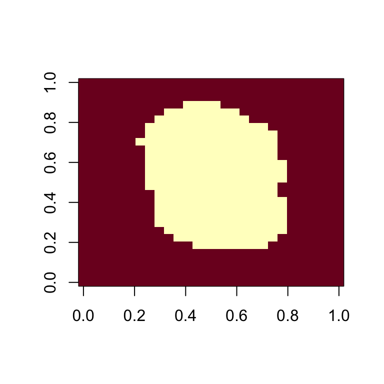
Preprocessing

So we end up removing

length(nzv)

[1] 532

predictors.

Preprocessing

The caret package features the preProcess function, which allows users to establish a predefined set of preprocessing operations based on a training set.
This function is designed to apply these operations to new datasets without recalculating anything on the test set, ensuring that all preprocessing steps are consistent and derived solely from the training data.

Preprocessing

Below is an example demonstrating how to remove predictors with near-zero variance and then center the remaining predictors:

pp <- preProcess(x, method = c("nzv", "center")) 
centered_subsetted_x_test <- predict(pp, newdata = x_test) 
dim(centered_subsetted_x_test)

[1] 1000  252

Additionally, the train function in caret includes a preProcess argument that allows users to specify which preprocessing steps to apply automatically during model training.

kNN

The first step is to optimize for $k$.

train_knn <- train(x, y, method = "knn",  
                   preProcess = "nzv", 
                   trControl = trainControl("cv", number = 20, p = 0.95), 
                   tuneGrid = data.frame(k = seq(1, 7, 2)))

kNN

Once we optimize our algorithm, the predict function defaults to using the best performing algorithm fit with the entire training data:

y_hat_knn <- predict(train_knn, x_test, type = "raw")

kNN

We achieve relatively high accuracy:

confusionMatrix(y_hat_knn, factor(y_test))$overall["Accuracy"]

Accuracy 
   0.952

The caret package

The caret package

The caret package

The caret package

The train function

The train function

The predict function

The predict function

The predict function

The predict function

The predict function

The predict function

The predict function

The predict function

The predict function

Resampling

The predict function

Resampling

Resampling

Resampling

Resampling

Resampling

Resampling

Resampling

Resampling

Resampling

Preprocessing

Preprocessing

Preprocessing

Preprocessing

Preprocessing

Preprocessing

Preprocessing

Preprocessing

Preprocessing

Preprocessing

Preprocessing

Preprocessing

kNN

kNN

kNN

The `train` function

The `train` function

The `predict` function

The `predict` function

The `predict` function

The `predict` function

The `predict` function

The `predict` function

The `predict` function

The `predict` function

The `predict` function

The `predict` function