Resampling Methods
2024-12-09
Resampling methods math
- Our goal is to find the \(\lambda\) that minimizes:
\[ \text{MSE}(\lambda) = \mbox{E}\{[\widehat{Y}(\lambda) - Y]^2 \} \]
- A intuitive first attempt is the apparent error defined by:
\[ \hat{\mbox{MSE}}(\lambda) = \frac{1}{N}\sum_{i = 1}^N \left\{\widehat{y}_i(\lambda) - y_i\right\}^2 \]
Resampling methods math
- But this is just one realization of a random variable.
\[ \hat{\mbox{MSE}}(\lambda) = \frac{1}{N}\sum_{i = 1}^N \left\{\widehat{y}_i(\lambda) - y_i\right\}^2 \]
- Can we find a better estimate?
Mathematical description of resampling methods
Imagine a world in which repeat data collection.
Take a large of number samples \(B\) define:
\[ \frac{1}{B} \sum_{b=1}^B \frac{1}{N}\sum_{i=1}^N \left\{\widehat{y}_i^b(\lambda) - y_i^b\right\}^2 \]
- Law of large numbers says this is close to \(MSE(\lambda)\).
Resampling methods math
We can’t do this in practice.
But we can try to immitate it.
Cross validation

Cross validation
Cross validation
K-fold cross validation
- Remember we are going to imitate this:
\[ \mbox{MSE}(\lambda) \approx\frac{1}{B} \sum_{b = 1}^B \frac{1}{N}\sum_{i = 1}^N \left(\widehat{y}_i^b(\lambda) - y_i^b\right)^2 \]
We want to generate a dataset that can be thought of as independent random sample, and do this \(B\) times.
The K in K-fold cross validation, represents the number of time \(B\).
K-fold cross validation
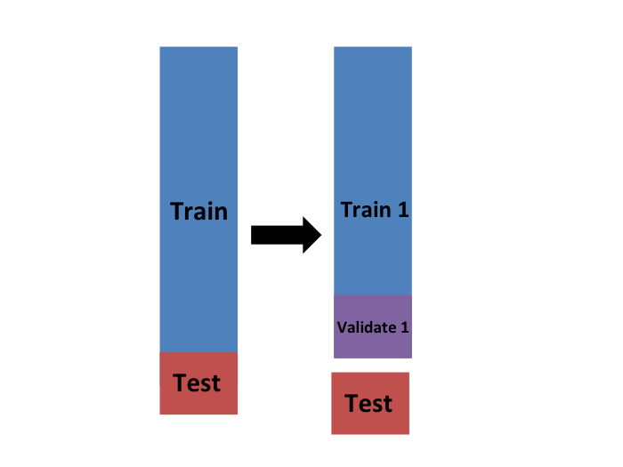
For each sample we simply pick \(M = N/B\) observations at random and think of these as a random sample \(y_1^b, \dots, y_M^b\), with \(b = 1\).
We call this the validation set.
Now we can fit the model in the training set, then compute the apparent error on the independent set:
\[ \hat{\mbox{MSE}}_b(\lambda) = \frac{1}{M}\sum_{i = 1}^M \left(\widehat{y}_i^b(\lambda) - y_i^b\right)^2 \]
K-fold cross validation
- In K-fold cross validation, we randomly split the observations into \(B\) non-overlapping sets:

K-fold cross validation
- Now we repeat the calculation above for each of these sets \(b = 1,\dots,B\) and obtain:
\[\hat{\mbox{MSE}}_1(\lambda),\dots, \hat{\mbox{MSE}}_B(\lambda)\]
- Then, for our final estimate, we compute the average:
\[ \hat{\mbox{MSE}}(\lambda) = \frac{1}{B} \sum_{b = 1}^B \hat{\mbox{MSE}}_b(\lambda) \]
K-fold cross validation
- A final step is to select the \(\lambda\) that minimizes the \(\hat{\mbox{MSE}}(\lambda)\).
\[ \hat{\mbox{MSE}}(\lambda) = \frac{1}{B} \sum_{b = 1}^B \hat{\mbox{MSE}}_b(\lambda) \]
How many folds?
How do we pick the cross validation fold?
Large values of \(B\) are preferable because the training data better imitates the original dataset.
However, larger values of \(B\) will have much slower computation time: for example, 100-fold cross validation will be 10 times slower than 10-fold cross validation.
For this reason, the choices of \(B = 5\) and \(B = 10\) are popular.
How many folds?
One way we can improve the variance of our final estimate is to take more samples.
To do this, we would no longer require the training set to be partitioned into non-overlapping sets.
Instead, we would just pick \(B\) sets of some size at random.
MSE of our optimized algorithm
We have described how to use cross validation to optimize parameters.
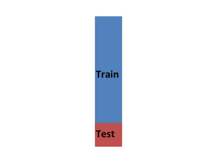
However, we now have to take into account the fact that the optimization occurred on the training data and we therefore need an estimate of our final algorithm based on data that was not used to optimize the choice.
Here is where we use the test set we separated early on.
MSE of our optimized algorithm

MSE of our optimized algorithm
- We can actually do cross validation again:

MSE of our optimized algorithm
and obtain a final estimate of our expected loss.
However, note that last cross validation iteration means that our entire compute time gets multiplied by \(K\).
You will soon learn that fitting each algorithm takes time because we are performing many complex computations.
As a result, we are always looking for ways to reduce this time.
For the final evaluation, we often just use the one test set.
MSE of our optimized algorithm
- Once we are satisfied with this model and want to make it available to others, we could refit the model on the entire dataset, without changing the optimized parameters.
MSE of our optimized algorithm

Boostrap resampling
Typically, cross-validation involves partitioning the original dataset into a training set to train the model and a testing set to evaluate it.
With the bootstrap approach you can create multiple different training datasets via bootstrapping.
This method is sometimes called bootstrap aggregating or bagging.
In bootstrap resampling, we create a large number of bootstrap samples from the original training dataset.
Boostrap resampling
Each bootstrap sample is created by randomly selecting observations with replacement, usually the same size as the original training dataset.
For each bootstrap sample, we fit the model and compute the MSE estimate on the observations not selected in the random sampling, referred to as the out-of-bag observations.
These out-of-bag observations serve a similar role to a validation set in standard cross-validation.
We then average the MSEs obtained in the out-of-bag observations.
Boostrap resampling
This approach is actually the default approach in the caret package.
We describe how to implement resampling methods with the caret package next.
Comparison of MSE estimates
