k-nearest neighbors (knn)
2024-12-10
Motivation
Motivation
- We are interested in estimating the conditional probability function:
\[ p(\mathbf{x}) = \mbox{Pr}(Y = 1 \mid X_1 = x_1, \dots, X_{784} = x_{784}). \]
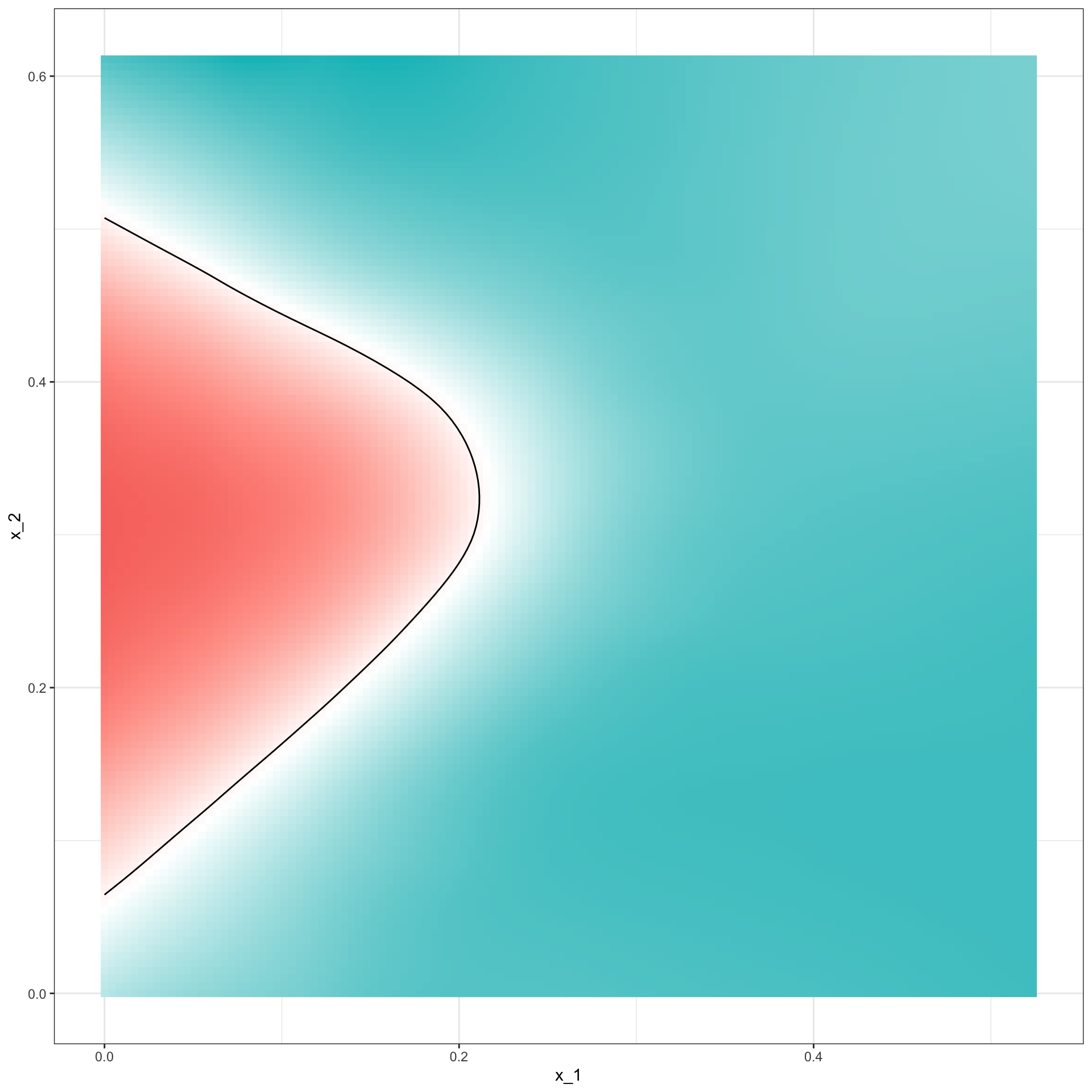
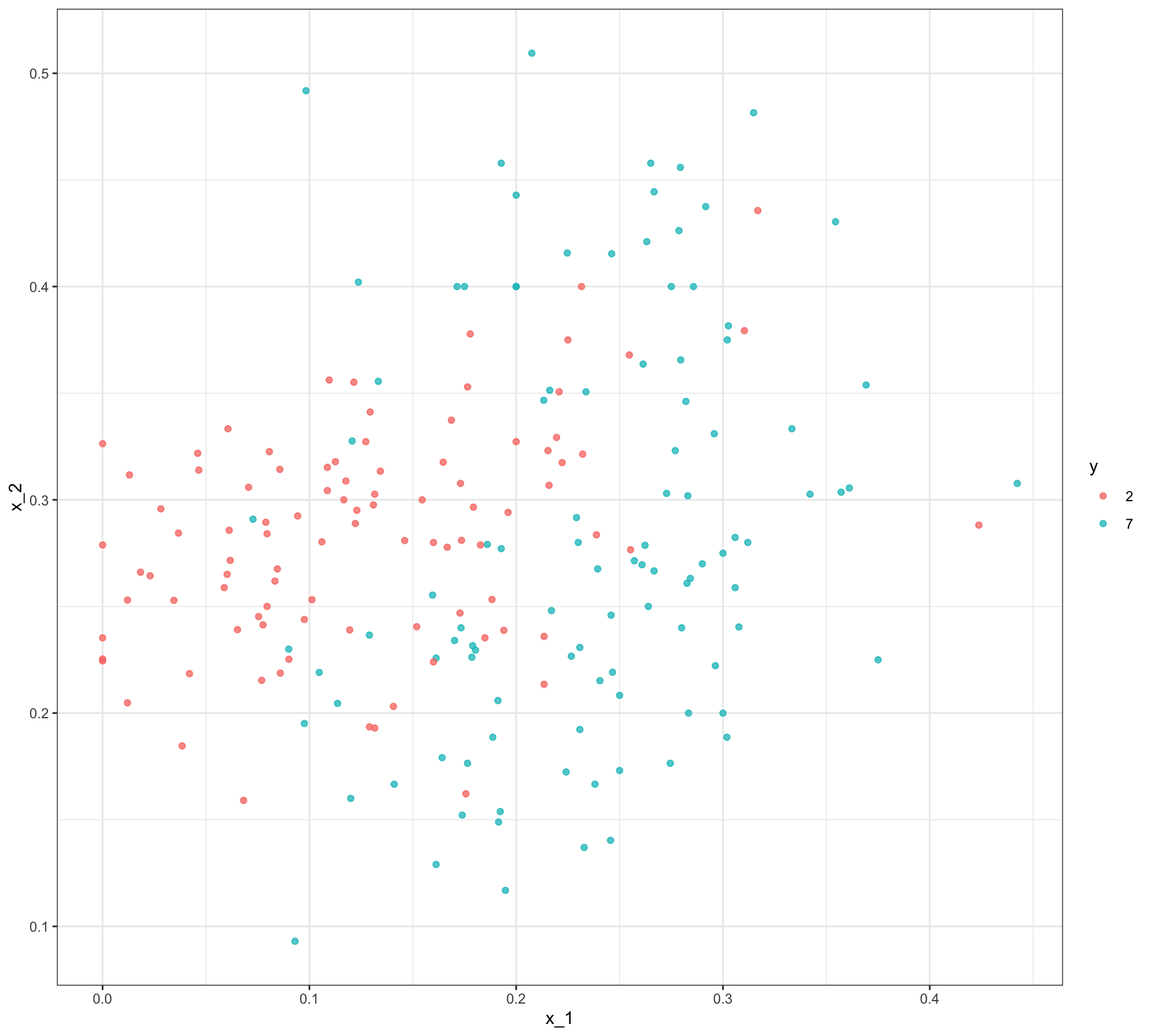
Simpler example
Conditional Probability Function
Motivation
- We are interested in estimating:
\[ p(\mathbf{x}) = \mbox{Pr}(Y = 1 \mid X_1 = x_1 , X_2 = x_2). \]
Training set
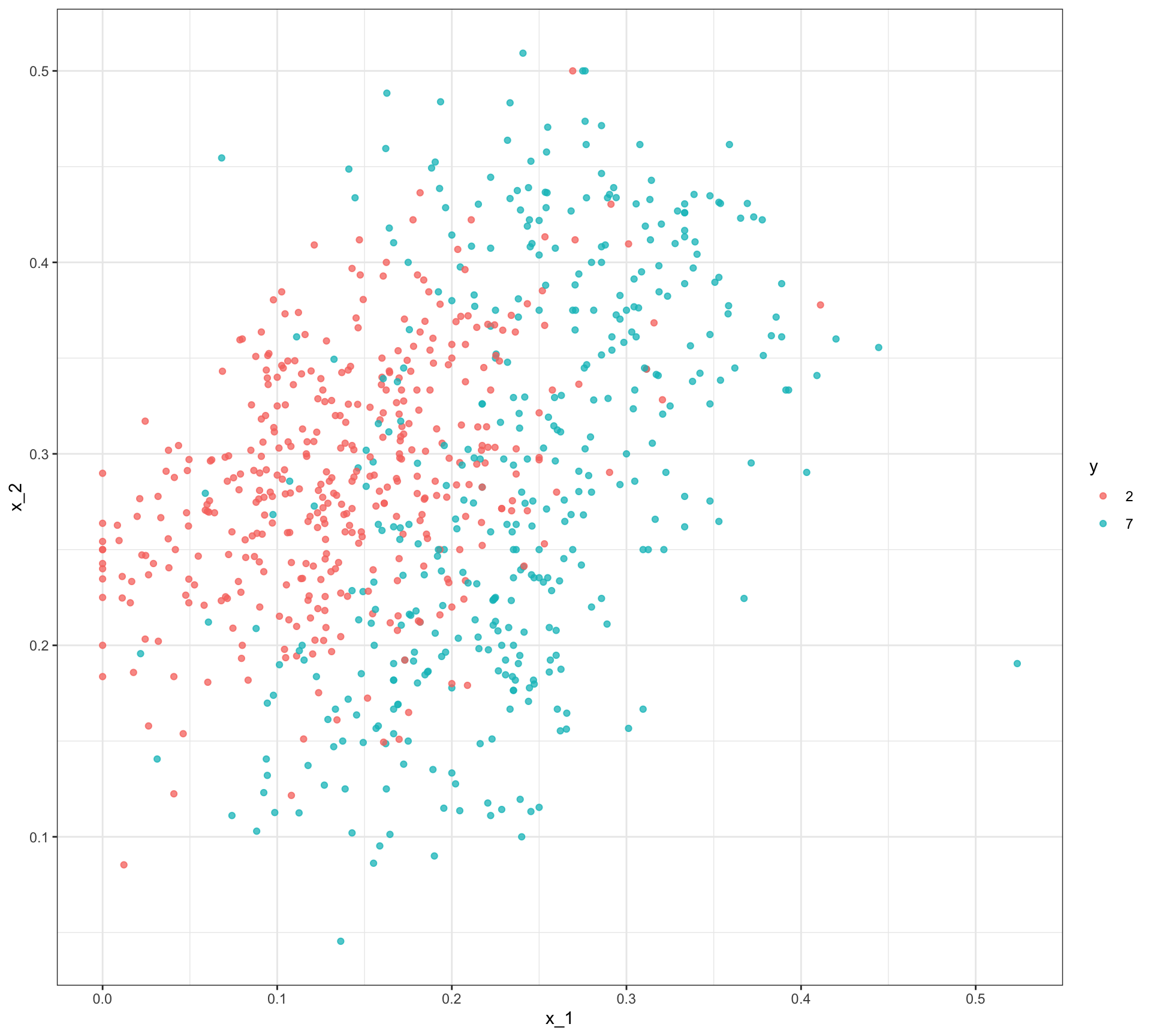
Test set
Motivation
With kNN we estimate \(p(\mathbf{x})\) using smoothing.
We define the distance between all observations based on the features.
For any \(\mathbf{x}_0\), we estimate \(p(\mathbf{x})\) by identifying the \(k\) nearest points to \(mathbf{x}_0\) and taking an average of the \(y\)s associated with these points.
We refer to the set of points used to compute the average as the neighborhood.
This gives us \(\widehat{p}(\mathbf{x}_0)\).
Motivation
As with bin smoothers, we can control the flexibility of our estimate through the \(k\) parameter: larger \(k\)s result in smoother estimates, while smaller \(k\)s result in more flexible and wiggly estimates.
To implement the algorithm, we can use the
knn3function from the caret package.Looking at the help file for this package, we see that we can call it in one of two ways.
We will use the first way in which we specify a formula and a data frame.
Let’s try it
kNN
This gives us \(\widehat{p}(\mathbf{x})\):
y_hat_knn <- predict(knn_fit, mnist_27$test, type = "class")
confusionMatrix(y_hat_knn, mnist_27$test$y)$overall["Accuracy"]
Accuracy
0.815 - We see that kNN, with the default parameter, already beats regression.
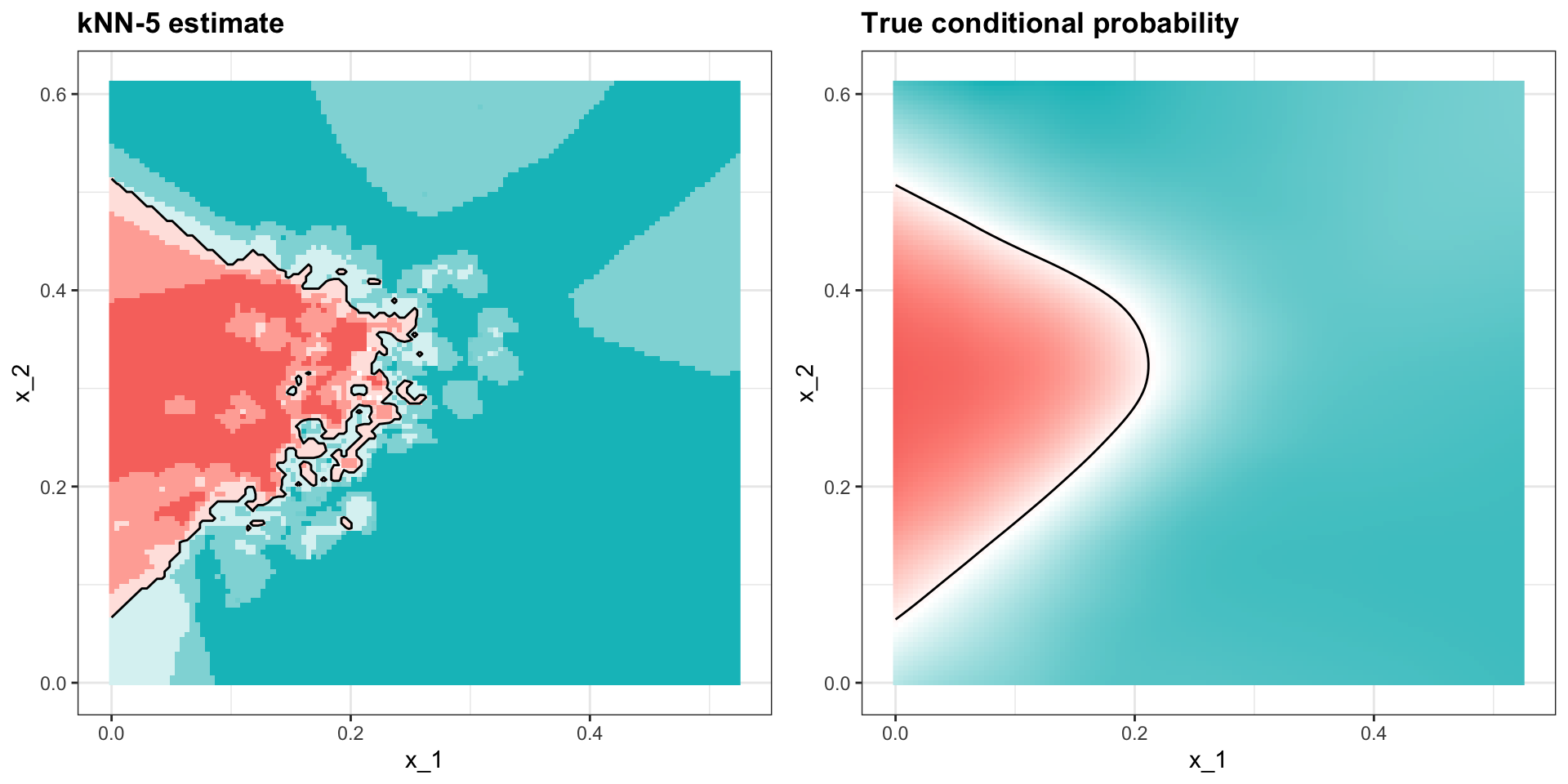
kNN
- To see why this is the case, we plot \(\widehat{p}(\mathbf{x})\) and compare it to the true conditional probability \(p(\mathbf{x})\):
Over-training
Compare
y_hat_knn <- predict(knn_fit, mnist_27$train, type = "class")
confusionMatrix(y_hat_knn, mnist_27$train$y)$overall["Accuracy"]
Accuracy
0.86 to
Over-training
Compare this:
knn_fit_1 <- knn3(y ~ ., data = mnist_27$train, k = 1)
y_hat_knn_1 <- predict(knn_fit_1, mnist_27$train, type = "class")
confusionMatrix(y_hat_knn_1, mnist_27$train$y)$overall[["Accuracy"]]
[1] 0.994to this:
y_hat_knn_1 <- predict(knn_fit_1, mnist_27$test, type = "class")
confusionMatrix(y_hat_knn_1, mnist_27$test$y)$overall["Accuracy"]
Accuracy
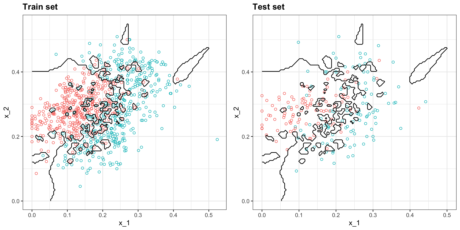
0.81 - We can see the over-fitting problem by plotting the decision rule boundaries produced by \(p(\mathbf{x})\):
Over-training
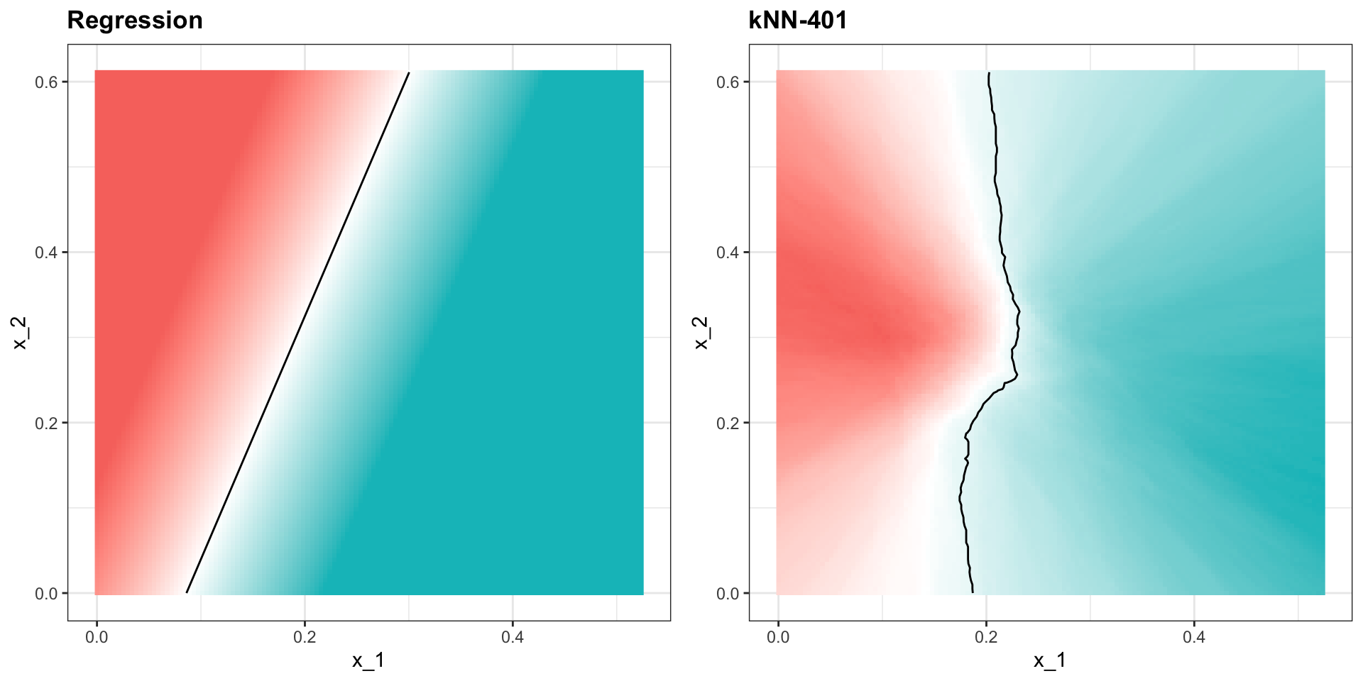
Over-smoothing
Let’s try a much bigger neighborhood:
Over-smoothing
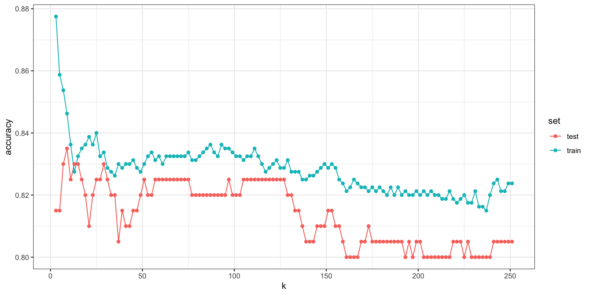
Parameter tuning