Treatment Effect Models

2024-11-12

Treatment effect models

Up to now, all our linear models have been applied to two or more continuous random variables.
We assume the random variables are multivariate normal and use this to motivate a linear model.
This approach covers many real-life examples of linear regression.

Treatment effect models

Linear models have many other applications.
One of the most popular is to quantify treatment effects in randomized and controlled experiments.
One of the first applications was in agriculture, where different plots of lands were treated with different combinations of fertilizers.
The use of \(Y\) for the outcome in statistics is due to the mathematical theory being developed for crop yield as the outcome.

Treatment effect models

The same ideas have been applied in other areas.
In randomized trials developed to determine if drugs cure or prevent diseases or if policies have an effect on social or educational outcomes.
We think of the policy intervention as a treatment so we can follow the same mathematical descriptions.
The analyses used in A/B testing are based on treatment effects models.

Definitions

Factors: Categorical variables used to define subgroups.
Levels: The distinct categories or groups within each factor.
Treatment: The factor we are interested in. Levels are often experimental and control.

Treatment effect models

These models have also been applied in observational studies as well.
We use linear models to estimate effects of interest while accounting for potential confounders.
For example, to estimate the effect of a diet high in fruits and vegetables on blood pressure, we would have to account for factors such as age, sex, and smoking status.

Case study

Mice were randomly selected and divided into two groups: one group receiving a high-fat diet while the other group served as the control.
The data is included in the dslabs package:

library(tidyverse) 
library(dslabs) 
table(mice_weights$diet)


chow   hf 
 394  386

Treatment effect models

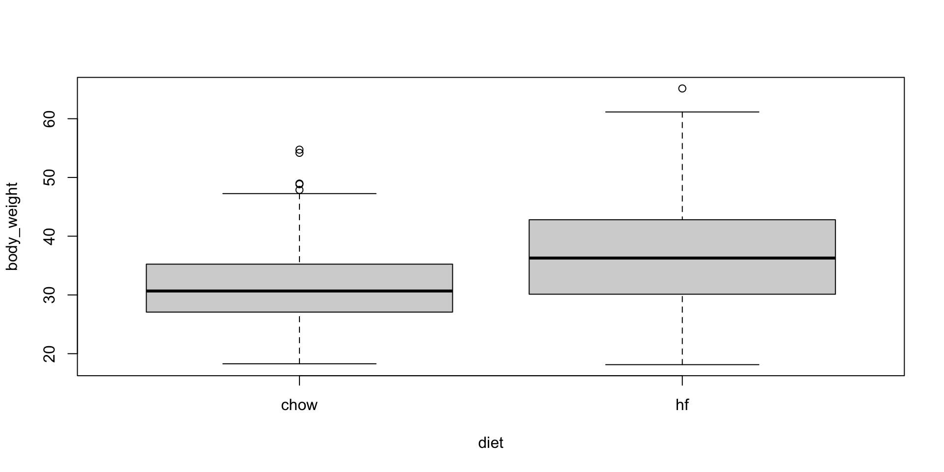
A boxplot shows that the high fat diet mice are, on average, heavier.

Comparing group means

Is it possible that the observed difference is simply due to chance?
We can apply the ideas we learned in the statistical inference lectures.
Define \(\mu_1\) and \(\mu_0\) the population averagees for treatment and control.
We want to know if \(\mu_1 - \mu_0 >0\).

Comparing group means

We know that the \(\bar{X}_1 - \bar{X}_0\)

mice_weights |> group_by(diet) |> summarize(average = mean(body_weight))

# A tibble: 2 × 2
  diet  average
  <fct>   <dbl>
1 chow     31.5
2 hf       36.7

follows a normal distribution, with expected value \(\mu_1-\mu_0\) and standard error:

\[ \sqrt{\frac{\sigma_1^2}{N_1} + \frac{\sigma_0^2}{N_0}} \]

Comparing group means

If we define the null hypothesis as the high-fat diet having no effect, or \(\mu_1 - \mu_0 = 0\), this implies that.

\[ \frac{\bar{X}_1 - \bar{X}_0}{\sqrt{\frac{\sigma_1^2}{N_1} + \frac{\sigma_0^2}{N_0}}} \]

has expected value 0 and standard error 1 and therefore approximately follows a standard normal distribution.

Comparing group means

Note that we can’t compute this quantity in practice because the \(\sigma_1\) and \(\sigma_0\) are unknown.
However, if we estimate them with the sample standard deviations the CLT still holds and:

\[ t = \frac{\bar{X}_1 - \bar{X}_0}{\sqrt{\frac{s_1^2}{N_1} + \frac{s_0^2}{N_0}}} \]

follows a standard normal distribution when the null hypothesis is true.

Comparing group means

This implies that we can easily compute the probability of observing a value as large as the one we obtained:

stats <- mice_weights |>  
  group_by(diet) |>  
  summarize(xbar = mean(body_weight), s = sd(body_weight), n = n())  
t_stat <- with(stats, (xbar[2] - xbar[1])/sqrt(s[2]^2/n[2] + s[1]^2/n[1])) 
t_stat

[1] 9.339096

Here \(t\) is well over 3, so we don’t really need to compute the p-value 1-pnorm(t_stat) as we know it will be very small.

Comparing group means

Note that when \(N\) is not large enough, then the CLT does not apply and we use the t-distribution:
So the calculation of the p-value is the same except that we use pt instead of pnorm.
Specifically, we use

1 - pt(t_stat, with(stats, n[2]+n[1]-2))

[1] 0

Warning

In the computation above, we computed the probability of t being as large as what we observed.
However, when our interest spans both directions, for example, either an increase or decrease in weight, we need to compute the probability of t being as extreme as what we observe.
The formula simply changes to using the absolute value: 1 - pnorm(abs(t-test)) or 1-pt(abs(t_stat), with(stats, n[2]+n[1]-2)).

One factor design

Although the t-test is useful for cases in which we compare two treatments, it is common to have other variables affect our outcomes.
For example, what if more male mice received the high-fat diet?
What if their is cage effect?
Linear models permit hypothesis testing in these more general situations.

One factor design

If we assume that the weight distributions for both chow and high-fat diets are normally distributed, we can write:

\[ Y_i = \beta_0 + \beta_1 x_i + \varepsilon_i \]

with \(X_i\) 1, if the \(i\)-th mice was fed the high-fat diet, and 0 otherwise, and the errors \(\varepsilon_i\) IID normal with expected value 0 and standard deviation \(\sigma\).

One factor design

Note that this mathematical formula looks exactly like the model we wrote out for the father-son heights.

\[ Y_i = \beta_0 + \beta_1 x_i + \varepsilon_i \]

\(x_i\) being 0 or 1 rather than a continuous variable, allows us to use it in this different context.
Now \(\beta_0\) represents the population average height of the mice on the chow diet and
\(\beta_0 + \beta_1\) represents the population average for the weight of the mice on the high-fat diet.

One factor design

A nice feature of this model is that \(\beta_1\) represents the treatment effect of receiving the high-fat diet.
The null hypothesis that the high-fat diet has no effect can be quantified as \(\beta_1 = 0\).

One factor design

A powerful characteristic of linear models is that we can estimate the \(\beta\)s and their standard errors with the same LSE machinery:

fit <- lm(body_weight ~ diet, data = mice_weights)

One factor design

Because diet is a factor with two entries, the lm function knows to fit the linear model above with a \(x_i\) a indicator variable.
The summary function shows us the resulting estimate, standard error, and p-value:

coefficients(summary(fit))

             Estimate Std. Error   t value     Pr(>|t|)
(Intercept) 31.537005  0.3858192 81.740369 0.000000e+00
diethf       5.136078  0.5484506  9.364705 8.021959e-20

One factor design

Using broom, we can write:

library(broom) 
tidy(fit, conf.int = TRUE) |> filter(term == "diethf")

# A tibble: 1 × 7
  term   estimate std.error statistic  p.value conf.low conf.high
  <chr>     <dbl>     <dbl>     <dbl>    <dbl>    <dbl>     <dbl>
1 diethf     5.14     0.548      9.36 8.02e-20     4.06      6.21

One factor design

The statistic computed here is the estimate divided by its standard error:

\[\hat{\beta}_1 / \hat{\mbox{SE}}(\hat{\beta}_1)\]

In the case of the simple one-factor model, we can show that this statistic is almost equivalent to the t-statistics computed in the previous section:

c(coefficients(summary(fit))[2,3], t_stat)

[1] 9.364705 9.339096

Note

In the linear model description provided here, we assumed \(\varepsilon\) follows a normal distribution.
This assumption permits us to show that the statistics formed by dividing estimates by their estimated standard errors follow t-distribution, which in turn allows us to estimate p-values or confidence intervals.
However, note that we do not need this assumption to compute the expected value and standard error of the least squared estimates.
Furthermore, if the number of observations is large enough, then the central limit theorem applies and we can obtain p-values and confidence intervals even without the normal distribution assumption for the errors.

Two factor designs

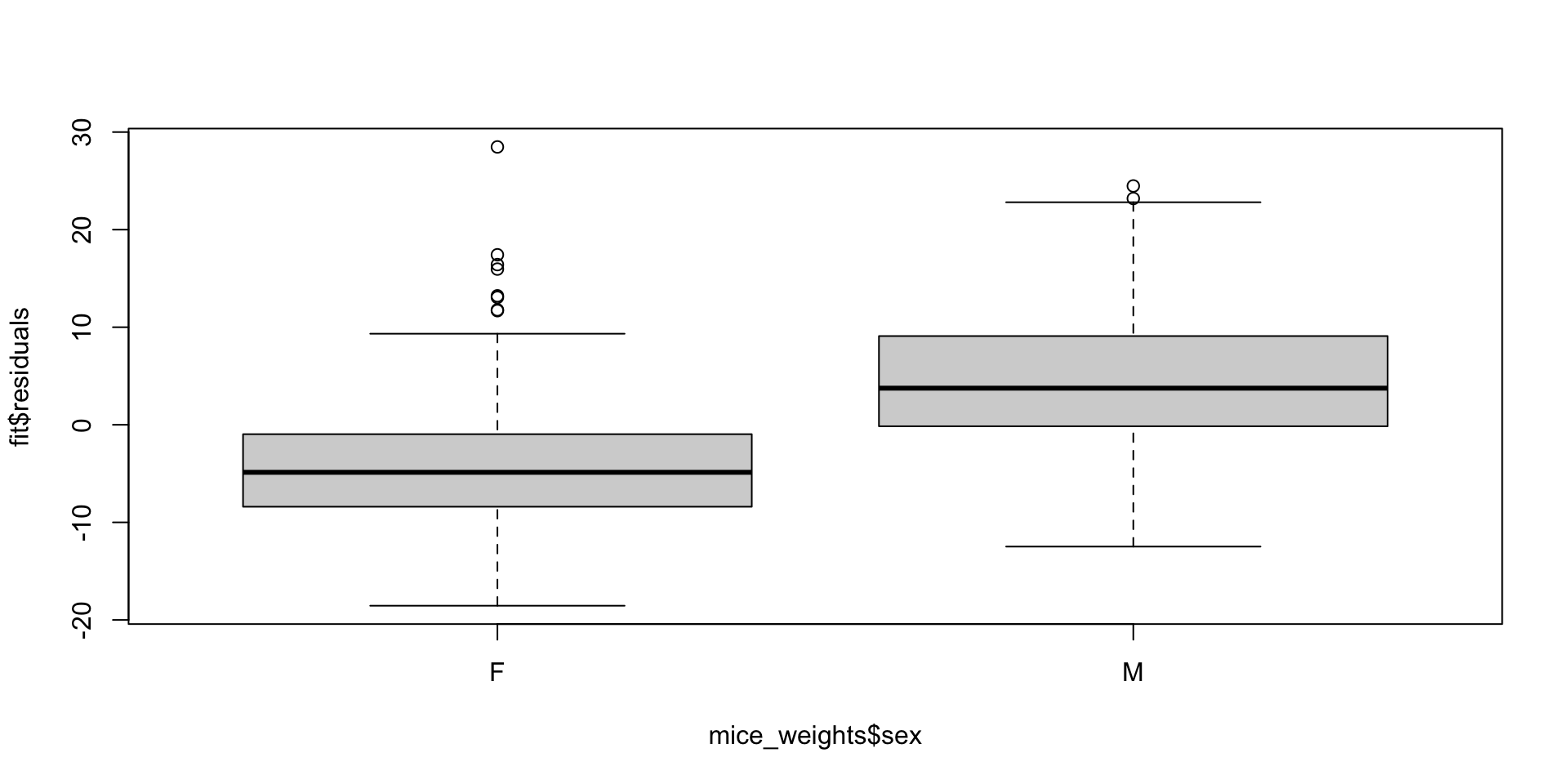
Note that this experiment included male and female mice, and male mice are known to be heavier.
This explains why the residuals depend on the sex variable:

boxplot(fit$residuals ~ mice_weights$sex)

Two factor designs

This misspecification can have real implications; for instance, if more male mice received the high-fat diet, then this could explain the increase.
Conversely, if fewer received it, we might underestimate the diet effect.
Sex could be a confounder, indicating that our model can certainly be improved.

Two factor designs

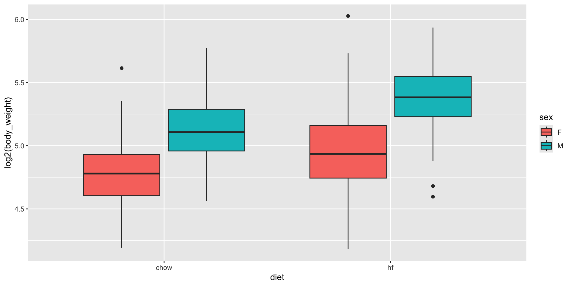
We can examine the data:

mice_weights |> ggplot(aes(diet, log2(body_weight), fill = sex)) + geom_boxplot()

Two factor designs

A linear model that permits a different expected value for the following four groups, 1) female on chow diet, 2) females on high-fat diet, 3) male on chow diet, and 4) males on high-fat diet, can be written like this:

\[ Y_i = \beta_1 x_{i,1} + \beta_2 x_{i,2} + \beta_3 x_{i,3} + \beta_4 x_{i,4} + \varepsilon_i \]

with \(x_{i,1},\dots,x_{i,4}\) indicator variables for each of the four groups.

Two factor designs

Note that with this representation we allow the diet effect to be different for males and females.
However, with this representation, none of the \(\beta\)s represent the effect of interest: the diet effect.
A powerful feature of linear models is that we can rewrite the model so that the expected value for each group remains the same, but the parameters represent the effects we are interested in.

Two factor designs

So, for example, in the representation.

\[ Y_i = \beta_0 + \beta_1 x_{i,1} + \beta_2 x_{i,2} + \beta_3 x_{i,1} x_{i,2} + \varepsilon_i \]

with \(x_{i,1}\) an indicator that is 1 if individual \(i\) is on the high-fat diet \(x_{i,2}\) an indicator that is 1 if you are male, the \(\beta_1\) is interpreted as the diet effect for females, \(\beta_2\) as the average difference between males and females, and \(\beta_3\) the difference in the diet effect between males and females.

Two factor designs

In statistics, \(\beta_3\) is referred to as an interaction effect.
The \(\beta_0\) is considered the baseline value, which is the average weight of females on the chow diet.

Two factor designs

Statistical textbooks describe several other ways in which the model can be rewritten to obtain other types of interpretations.
For example, we might want \(\beta_2\) to represent the overall diet effect (the average between female and male effect) rather than the diet effect on females.

Two factor designs

This is achieved by defining what contrasts we are interested in.
In R, we can specific the linear model above using the following:

fit <- lm(body_weight ~ diet*sex, data = mice_weights)

The * implies that the term that multiplies \(x_{i,1}\) and \(x_{i,2}\) should be included, along with the \(x_{i,1}\) and \(x_{i,2}\) terms.

Two factor designs

Here are the estimates:

tidy(fit, conf.int = TRUE) |> filter(!str_detect(term, "Intercept"))

# A tibble: 3 × 7
  term        estimate std.error statistic  p.value conf.low conf.high
  <chr>          <dbl>     <dbl>     <dbl>    <dbl>    <dbl>     <dbl>
1 diethf          3.88     0.624      6.22 8.02e-10    2.66       5.10
2 sexM            7.53     0.627     12.0  1.27e-30    6.30       8.76
3 diethf:sexM     2.66     0.891      2.99 2.91e- 3    0.912      4.41

Note that the male effect is larger that the diet effect, and the diet effect is statistically significant for both sexes, with diet affecting males more by between 1 and 4.5 grams.

Two factor designs

A common approach applied when more than one factor is thought to affect the measurement is to simply include an additive effect for each factor, like this:

\[ Y_i = \beta_0 + \beta_1 x_{i,1} + \beta_2 x_{i,2} + \varepsilon_i \]

In this model, the \(\beta_1\) is a general diet effect that applies regardless of sex.

Two factor designs

In R, we use the following code, employing a + instead of *:

fit <- lm(body_weight ~ diet + sex, data = mice_weights)

Note that this model does not account for the difference in diet effect between males and females.

Two factor designs

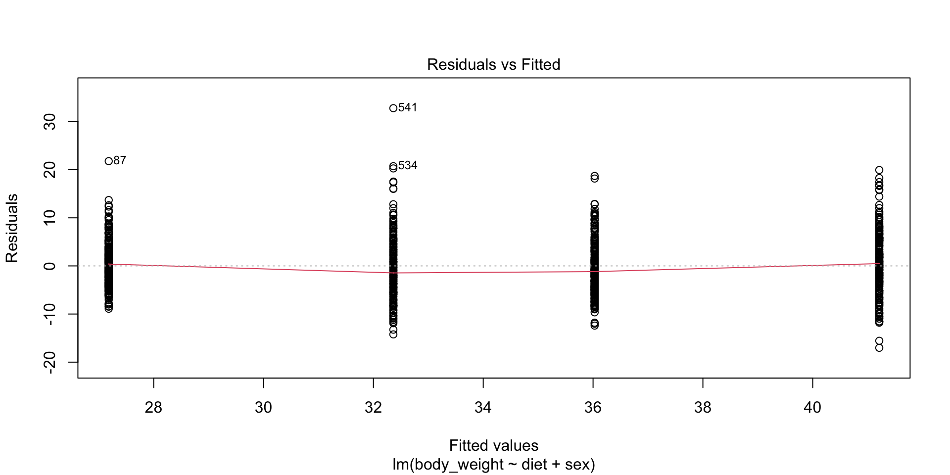
Diagnostic plots would reveal this deficiency by showing that the residuals are biased: they are, on average, negative for females on the diet and positive for males on the diet, rather than being centered around 0.

plot(fit, which = 1)

Two factor designs

Scientific studies, particularly within epidemiology and social sciences, frequently omit interaction terms from models due to the high number of variables.
Adding interactions necessitates numerous parameters, which in extreme cases may prevent the model from fitting.
However, this approach assumes that the interaction terms are zero, and if incorrect, it can skew the interpretation of the results.
Conversely, when this assumption is valid, models excluding interactions are simpler to interpret, as parameters are typically viewed as the extent to which the outcome increases with the assigned treatment.

Tip

Linear models are highly flexible and applicable in many contexts.
For example, we can include many more factors than just 2.
We have only just scratched the surface of how linear models can be used to estimate treatment effects.
We highly recommend learning more about this by exploring linear model textbooks and R manuals that cover the use of functions such as lm, contrasts, and model.matrix.

Contrasts

In the examples we have examined, each treatment had only two groups: diet had chow/high-fat, and sex had female/male.
However, variables of interest often have more than one level.
For example, we might have tested a third diet on the mice.
In statistics textbooks, these variables are referred to as a factor, and the groups in each factor are called its levels.

Contrasts

When a factor is included in the formula, the default behavior for lm is to define the intercept term as the expected value for the first level, and the other coefficient are to represent the difference, or contrast, between the other levels and first.
We can see when we estimate the sex effect with lm like this:

fit <- lm(body_weight ~ sex, data = mice_weights) 
coefficients(fit)

(Intercept)        sexM 
  29.758844    8.820658

Contrasts

To recover the expected mean for males, we can simply add the two coefficients:

sum(fit$coefficients[1:2])

[1] 38.5795

The package emmeans simplifies the calculation and also calculates standard errors:

library(emmeans) 
emmeans(fit, ~sex)

 sex emmean    SE  df lower.CL upper.CL
 F     29.8 0.339 778     29.1     30.4
 M     38.6 0.346 778     37.9     39.3

Confidence level used: 0.95

Contrasts

Now, what if we really didn’t want to define a reference level? What if we wanted a parameter to represent the difference from each group to the overall mean? Can we write a model like this:

\[ Y_i = \beta_0 + \beta_1 x_{i,1} + \beta_2 x_{i,2} + \varepsilon_i \]

with \(x_{i,1} = 1\), if observation \(i\) is female and 0 otherwise, and \(x_{i,2}=1\), if observation \(i\) is male and 0 otherwise?

Contrasts

Unfortunately, this representation has a problem.
Note that the mean for females and males are represented by \(\beta_0 + \beta_1\) and \(\beta_0 + \beta_2\), respectively.
This is a problem because the expected value for each group is just one number, say \(\mu_f\) and \(\mu_m\), and there is an infinite number of ways \(\beta_0 + \beta_1 = \mu_f\) and \(\beta_0 +\beta_2 = \mu_m\) (three unknowns with two equations).
This implies that we can’t obtain a unique least squares estimates.
The model, or parameters, are unidentifiable.

Contrasts

The default behavior in R solves this problem by requiring \(\beta_1 = 0\), forcing \(\beta_0 = \mu_m\), which permits us to solve the system of equations.
Keep in mind that this is not the only constraint that permits estimation of the parameters.

Contrasts

Any linear constraint will do as it adds a third equation to our system.
A widely used constraint is to require \(\beta_1 + \beta_2 = 0\).
To achieve this in R, we can use the argument contrast in the following way:

fit <- lm(body_weight ~ sex, data = mice_weights,  
          contrasts = list(sex = contr.sum)) 
coefficients(fit)

(Intercept)        sex1 
  34.169173   -4.410329

Contrasts

We see that the intercept is now larger, reflecting the overall mean rather than just the mean for females.
The other coefficient, \(\beta_1\), represents the contrast between females and the overall mean in our model.
The coefficient for men is not shown because it is redundant: \(\beta_1= -\beta_2\).

Contrasts

If we want to see all the estimates, the emmeans package also makes the calculations for us:

contrast(emmeans(fit, ~sex))

 contrast estimate    SE  df t.ratio p.value
 F effect    -4.41 0.242 778 -18.203  <.0001
 M effect     4.41 0.242 778  18.203  <.0001

P value adjustment: fdr method for 2 tests

Contrasts

The use of this alternative constraint is more practical when a factor has more than one level, and choosing a baseline becomes less convenient.
Furthermore, we might be more interested in the variance of the coefficients rather than the contrasts between groups and the reference level.

Contrasts

As an example, consider that the mice in our dataset are actually from several generations:

table(mice_weights$gen)


  4   7   8   9  11 
 97 195 193  97 198

Contrasts

To estimate the variability due to the different generations, a convenient model is:

\[ Y_i = \beta_0 + \sum_{j=1}^J \beta_j x_{i,j} + \varepsilon_i \]

with \(x_{i,j}\) indicator variables: \(x_{i,j}=1\) if mouse \(i\) is in level \(j\) and 0 otherwise, \(J\) representing the number of levels, in our example 5 generations, and the level effects constrained with.

\[ \frac{1}{J} \sum_{j=1}^J \beta_j = 0 \implies \sum_{j=1}^J \beta_j = 0. \]

Contrasts

The constraint makes the model identifiable and also allows us to quantify the variability due to generations with:

\[ \sigma^2_{\text{gen}} \equiv \frac{1}{J}\sum_{j=1}^J \beta_j^2 \]

Contrasts

We can see the estimated coefficients using the following:

fit <- lm(body_weight ~ gen,  data = mice_weights,  
          contrasts = list(gen = contr.sum)) 
contrast(emmeans(fit, ~gen))

 contrast     estimate    SE  df t.ratio p.value
 gen4 effect    -0.122 0.705 775  -0.174  0.8621
 gen7 effect    -0.812 0.542 775  -1.497  0.3372
 gen8 effect    -0.113 0.544 775  -0.207  0.8621
 gen9 effect     0.149 0.705 775   0.212  0.8621
 gen11 effect    0.897 0.540 775   1.663  0.3372

P value adjustment: fdr method for 5 tests

Analysis of variance (ANOVA)

When a factor has more than one level, it is common to want to determine if there is significant variability across the levels rather than specific difference between any given pair of levels.
Analysis of variances (ANOVA) provides tools to do this.
ANOVA provides an estimate of \(\sigma^2_{\text{gen}}\) and a statistical test for the null hypothesis that the factor contributes no variability: \(\sigma^2_{\text{gen}} =0\).
Once a linear model is fit using one or more factors, the aov function can be used to perform ANOVA.

Analysis of variance (ANOVA)

Specifically, the estimate of the factor variability is computed along with a statistic that can be used for hypothesis testing:

summary(aov(fit))

             Df Sum Sq Mean Sq F value Pr(>F)
gen           4    294   73.50   1.128  0.342
Residuals   775  50479   65.13

Analysis of variance (ANOVA)

Keep in mind that if given a model formula, aov will fit the model:

summary(aov(body_weight ~ gen, data = mice_weights))

We do not need to specify the constraint because ANOVA needs to constrain the sum to be 0 for the results to be interpretable.
This analysis indicates that generation is not statistically significant.

Note

We do not include many details, for example, on how the summary statistics and p-values shown by aov are defined and motivated.
There are several books dedicated to the analysis of variance, and textbooks on linear models often include chapters on this topic.
Those interested in learning more about these topics can consult one of these textbooks.

Multiple factors

ANOVA was developed to analyze agricultural data, which included several factors.
We can perform ANOVA with multiple factors:

summary(aov(body_weight ~ sex + diet + gen,  data = mice_weights))

             Df Sum Sq Mean Sq F value Pr(>F)    
sex           1  15165   15165 389.799 <2e-16 ***
diet          1   5238    5238 134.642 <2e-16 ***
gen           4    295      74   1.895  0.109    
Residuals   773  30074      39                   
---
Signif. codes:  0 '***' 0.001 '**' 0.01 '*' 0.05 '.' 0.1 ' ' 1

This analysis suggests that sex is the biggest source of variability, which is consistent with previously made exploratory plots.

Warning

One of the key aspects of ANOVA (Analysis of Variance) is its ability to decompose the total variance in the data, represented by \(\sum_{i=1}^n Y_i^2\), into individual contributions attributable to each factor in the study.
However, for the mathematical underpinnings of ANOVA to be valid, the experimental design must be balanced.
This means that for every level of any given factor, there must be an equal representation of the levels of all other factors.
In our study involving mice, the design is unbalanced, requiring a cautious approach in the interpretation of the ANOVA results.

Array representation

When the model includes more than one factor, writing down linear models can become cumbersome.

Array representation

For example, in our two factor model, we include indicator variables for both factors:

\[ Y_i = \beta_0 + \sum_{j=1}^J \beta_j x_{i,j} + \sum_{k=1}^K \beta_{J+k} x_{i,J+k} + \varepsilon_i \\ \mbox{ with }\sum_{j=1}^J \beta_j=0 \mbox{ and } \sum_{k=1}^K \beta_{J+k} = 0, \]

the \(x\)s are indicator functions for the different levels.

Array representation

Specifically, in

\[ Y_i = \beta_0 + \sum_{j=1}^J \beta_j x_{i,j} + \sum_{k=1}^K \beta_{J+k} x_{i,J+k} + \varepsilon_i \]

the \(x_{i,1},\dots,x_{i,J}\) indicator functions for the \(J\) levels in the first factor and \(x_{i,J+1},\dots,x_{i,J+K}\) indicator functions for the \(K\) levels in the second factor.

Array representation

An alternative approach widely used in ANOVA to avoid indicators variables, is to save the data in an array, using different Greek letters to denote factors and indices to denote levels:

\[ Y_{i,j,k} = \mu + \alpha_j + \beta_k + \varepsilon_{i,j,k} \]

with \(\mu\) the overall mean, \(\alpha_j\) the effect of level \(j\) in the first factor, and \(\beta_k\) the effect of level \(k\) in the second factor.

Array representation

The constraint can now be written as:

\[ \sum_{j=1}^J \alpha_j = 0 \text{ and } \sum_{k=1}^K \beta_k = 0 \]

This notation lends itself to estimating the effects by computing means across dimensions of the array.