Hierarchical Models

2024-10-30

Hierarchichal Models

Hierarchical models are useful for quantifying different levels of variability or uncertainty.
One can use them using a Bayesian or Frequentist framework.
We illustrate the use of hierarchical models with an example from election forecasting. In this context, hierarchical modeling helps to manage expectations by accounting for various levels of uncertainty including polling biases that change direction from election to election.

Case study: election forecasting

In 2016, most forecasters underestimated Trump’s chances of winning greatly.
The day before the election, the New York Times reported the following probabilities for Hillary Clinton winning the presidency:

	NYT	538	HuffPost	PW	PEC	DK	Cook	Roth
Win Prob	85%	71%	98%	89%	>99%	92%	Lean Dem	Lean Dem

Case study: election forecasting

Note that FiveThirtyEight had Trump’s probability of winning at 29%, substantially higher than the others.
In fact, four days before the election, FiveThirtyEight published an article titled Trump Is Just A Normal Polling Error Behind Clinton.
So why did FiveThirtyEight’s model fair so much better than others?

Case study: election forecasting

For illustrative purposes, we will continue examining the popular vote example.
At the end we will describe a more complex approach used to forecast the electoral college result.

The general bias

We previously computed the posterior probability of Hillary Clinton winning the popular vote with a standard Bayesian analysis and found it to be very close to 100%.
However, FiveThirtyEight gave her a 81.4% chance.
What explains this difference?

The general bias

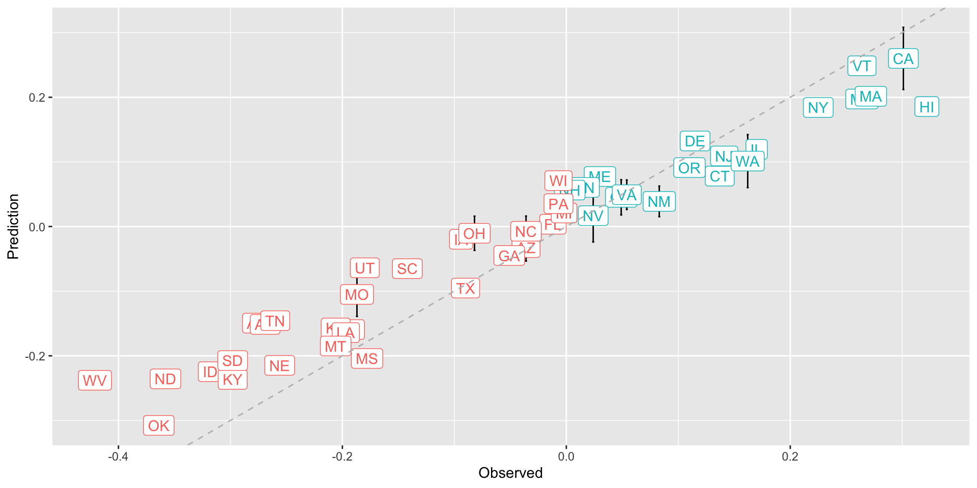
After elections are over, one can look at the difference between the pollster predictions and the actual result.
An important observation, that our initial models did not take into account, is that it is common to see a general bias that affects most pollsters in the same way, making the observed data correlated.

The general bias

Predicted versus observed:

The general bias

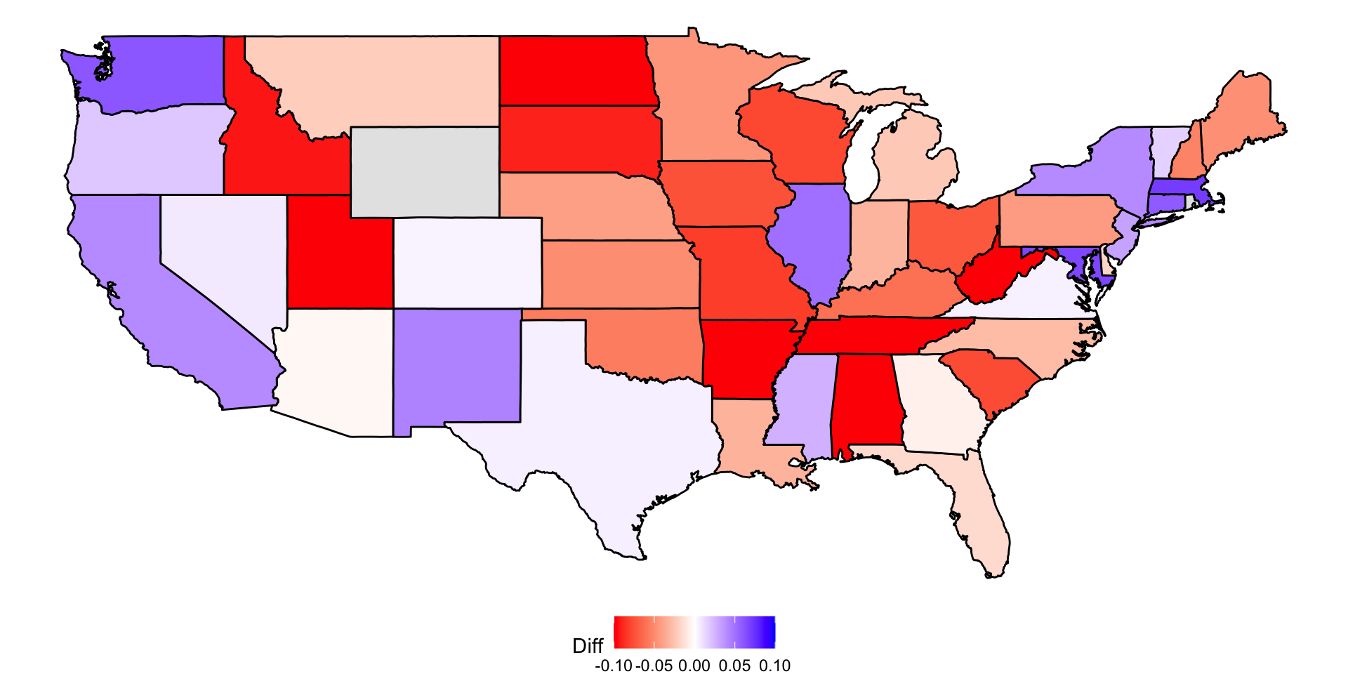
There is no agreed upon explanation for this, but we do observe it in historical data: in one election, the average of polls favors Democrats by 2%; then in the following election, they favor Republicans by 1%; then in the next election there is no bias; then in the following one Republicans are favored by 3%, …
There appears to be regional effect, not included in our analysis.

The general bias

In 2016, the polls were biased in favor of the Democrats by 2-3%.
Although we know this bias term affects our polls, we have no way of knowing what this bias is until election night.
So we can’t correct our polls accordingly.
What we can do is include a term in our model that accounts for the variability.

Hierarchical model

Suppose we are collecting data from one pollster and we assume there is no general bias.
The pollster collects several polls with a sample size of \(N\), so we observe several measurements of the spread \(X_1, \dots, X_J\).
Suppose the real proportion for Hillary is \(p\) and the difference is \(\mu\).

Hierarchical model

The urn model theory tells us that:

\[ X_j \sim \mbox{N}\left(\mu, 2\sqrt{p(1-p)/N}\right) \]

We use the index \(j\) to represent the different polls conducted by this pollster.

Hierarchical model

Here is a simulation for six polls assuming the spread is 2.1 and \(N\) is 2,000:

set.seed(3) 
J <- 6 
N <- 2000 
mu <- .021 
p <- (mu + 1)/2 
X <- rnorm(J, mu, 2*sqrt(p*(1 - p)/N))

Hierarchical model

Now, suppose we have \(J=6\) polls from each of \(I=5\) different pollsters.
For simplicity, let’s say all polls had the same sample size \(N\).
The urn model tell us the distribution is the same for all pollsters, so to simulate data, we use the same model for each:

I <- 5 
J <- 6 
N <- 2000 
X <- sapply(1:I, function(i){ 
  rnorm(J, mu, 2*sqrt(p*(1 - p)/N)) 
})

Hierarchical model

As expected, the simulated data does not really seem to capture the features of the actual data because it does not account for pollster-to-pollster variability:

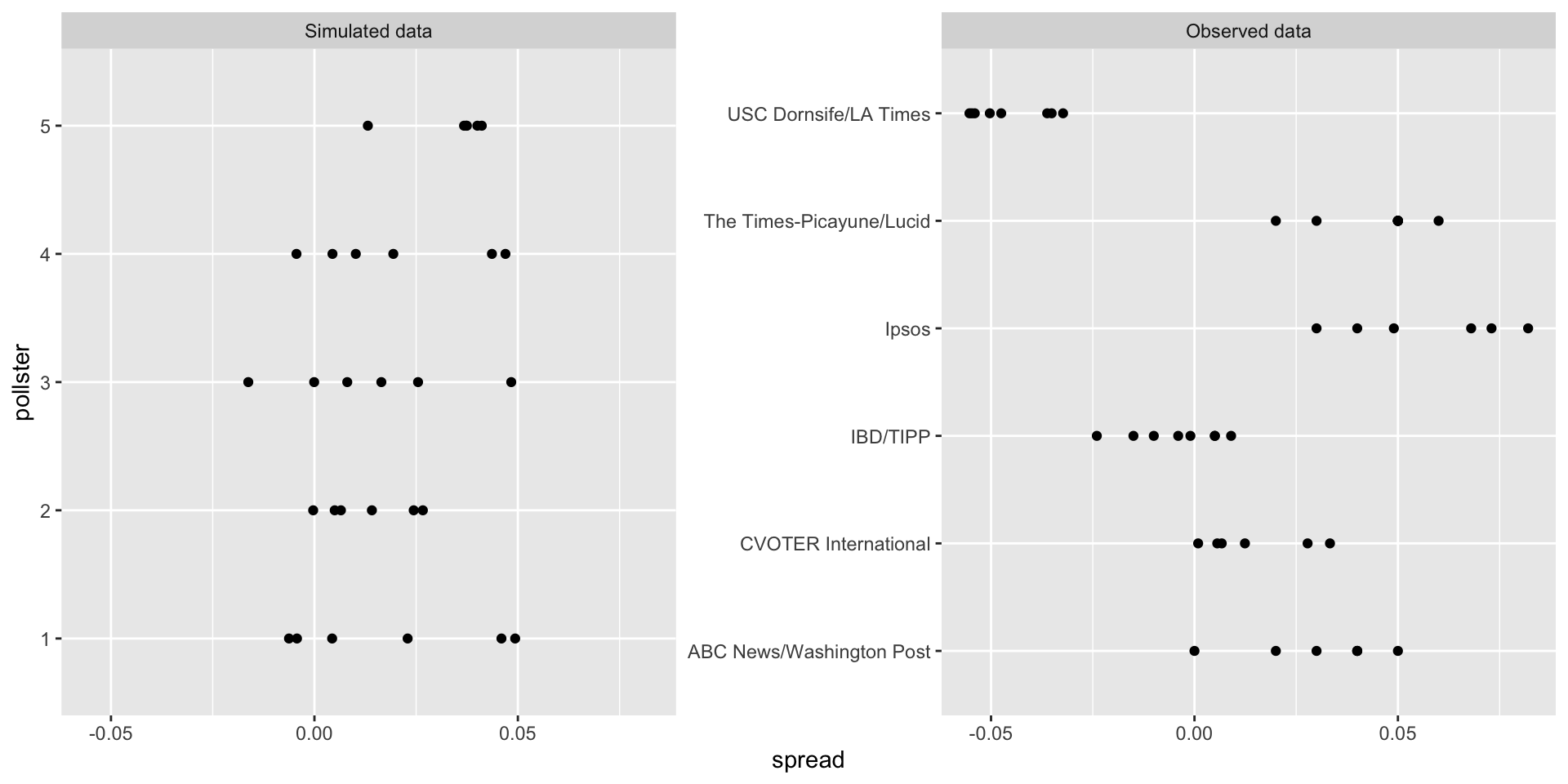
Hierarchical model

To fix this, we need to represent the two levels of variability and we need two indexes, one for pollster and one for the polls each pollster takes.
We use \(X_{ij}\) with \(i\) representing the pollster and \(j\) representing the \(j\)-th poll from that pollster.

Hierarchical model

The model is now augmented to include pollster effects \(h_i\), referred to as “house effects” by FiveThirtyEight, with standard deviation \(\sigma_h\):

\[ \begin{aligned} h_i &\sim \mbox{N}\left(0, \sigma_h\right)\\ X_{i,j} \mid h_i &\sim \mbox{N}\left(\mu + h_i, \sqrt{p(1-p)/N}\right) \end{aligned} \]

Hierarchical model

To simulate data from a specific pollster, we first need to draw an \(h_i\), and then generate individual poll data after adding this effect.
Here is how we would do it for one specific pollster (we assume \(\sigma_h\) is 0.025):

I <- 5 
J <- 6 
N <- 2000 
mu <- .021 
p <- (mu + 1)/2 
h <- rnorm(I, 0, 0.025) 
X <- sapply(1:I, function(i){ 
  mu + h[i] + rnorm(J, 0, 2*sqrt(p*(1 - p)/N)) 
})

Hierarchical model

The simulated data now looks more like the actual data:

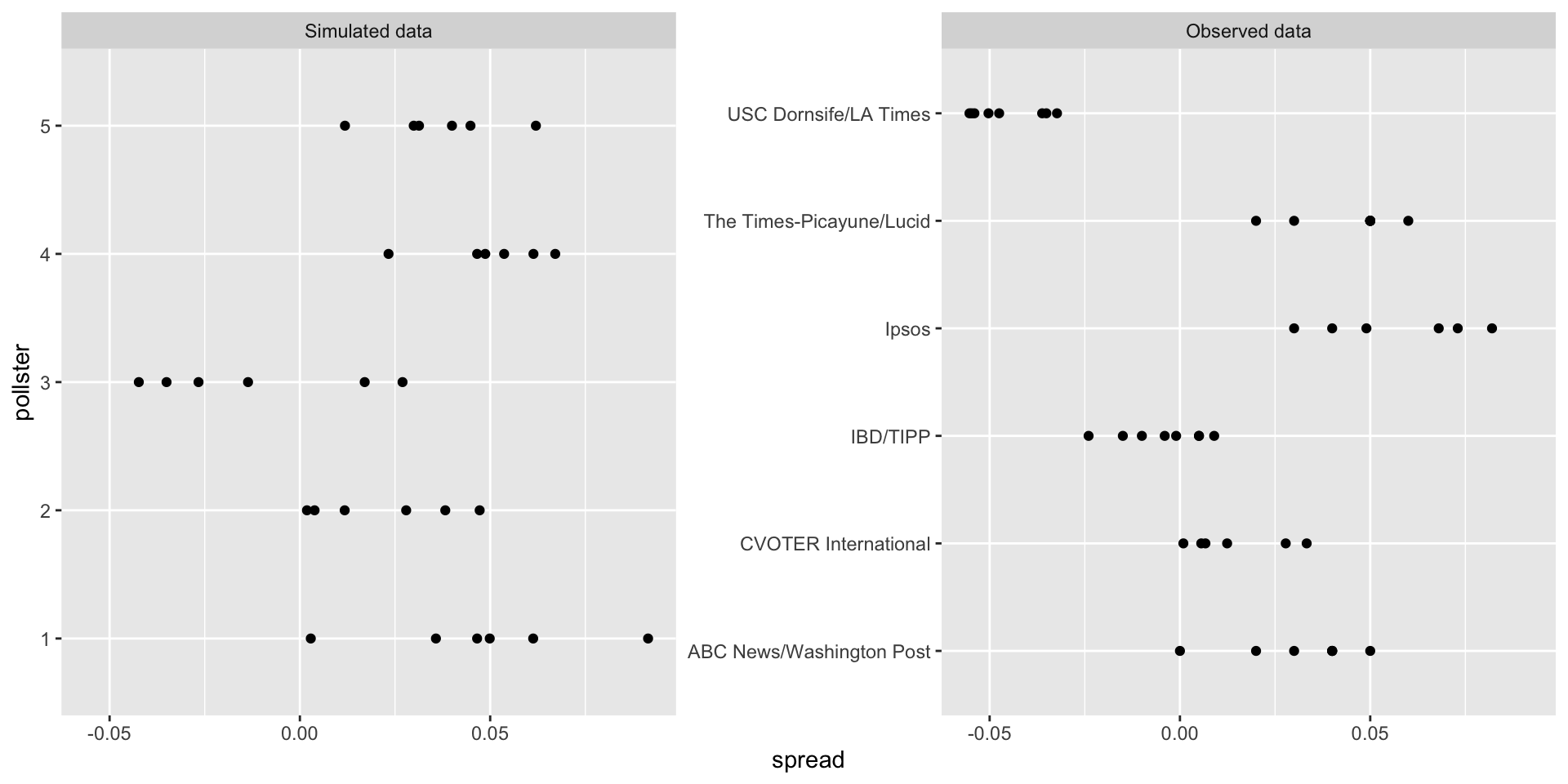
Hierarchical model

Note that \(h_i\) is common to all the observed spreads from a specific pollster.
Different pollsters have a different \(h_i\), which explains why we can see the groups of points shift up and down from pollster to pollster.
Now, in this model, we assume the average pollster effect is 0.
We think that for every pollster biased in favor of our party, there is another one in favor of the other, and assume the standard deviation is \(\sigma_h\).

Hierarchical model

But, historically, we see that every election has a general bias affecting all polls.
We can observe this with the 2016 data.
If we collect historical data, we see that the average of polls misses by more than models like the one above predict.
To see this, we would take the average of polls for each election year and compare it to the actual value.
If we did this, we would see a difference with a standard deviation of between 2-3%.

Hierarchical model

To account for this variability we can add another level to the model as follows:

\[ \begin{aligned} b &\sim \mbox{N}\left(0, \sigma_b\right)\\ h_j \mid \, b &\sim \mbox{N}\left(b, \sigma_h\right)\\ X_{i,j} | \, h_j, b &\sim \mbox{N}\left(\mu + h_j, \sqrt{p(1-p)/N}\right) \end{aligned} \]

Hierarchical model

This model accounts for three levels of variability:

Variability in the bias observed from election to election, quantified by \(\sigma_b\).
Pollster-to-pollster or house effect variability, quantified by \(\sigma_h\).
Poll sampling variability, which we can derive to be \(\sqrt(p(1-p)/N)\).

Hierarchical model

Note that not including a term like \(b\) in the models is what led many forecasters to be overconfident.
This random variable changes from election to election, but for any given election, it is the same for all pollsters and polls within one election.
This implies that we can’t estimate \(\sigma_h\) with data from just one election.
It also implies that the random variables \(X_{i,j}\) for a fixed election year share the same \(b\) and are therefore correlated.

Hierarchical model

One way to interpret \(b\) is as the difference between the average of all polls from all pollsters and the actual result of the election.
Since we don’t know the actual result until after the election, we can’t estimate \(b\) until then.

Warning

Some of the results presented in this section rely on calculations of the statistical properties of summaries based on correlated random variables.
To learn about the related mathematical details we skip in this book, please consult a textbook on hierarchical models:

Computing a posterior

Now, let’s fit the model above to data:

polls <- polls_us_election_2016 |>  
  filter(state == "U.S." & enddate >= "2016-10-31" & 
           (grade %in% c("A+","A","A-","B+", "B"))) |>  
  mutate(spread = rawpoll_clinton/100 - rawpoll_trump/100)

Computing a posterior

Here, we have just one poll per pollster, so we will drop the \(j\) index and represent the data as before with \(X_1, \dots, X_I\).

one_poll_per_pollster <- polls |> group_by(pollster) |>  
  filter(enddate == max(enddate)) |> 
  ungroup()

Computing a posterior

As a reminder, we have data from \(I=15\) pollsters.
Based on the model assumptions described above, we can mathematically show that the average \(\bar{X}\):

x_bar <- mean(one_poll_per_pollster$spread)

this has expected value \(\mu\).
But how precise is this estimate?

Computing a posterior

Because the \(X_i\) are correlated, estimating the standard error is more complex than what we have described up to now.
Specifically, using advanced statistical calculations not shown here, we can show that the typical variance (standard error squared) estimate:

s2 <- with(one_poll_per_pollster, sd(spread)^2/length(spread))

will consistently underestimate the true standard error by about \(\sigma_b^2\).
To estimate \(\sigma_b\), we need data from several elections.

Computing a posterior

By collecting and analyzing polling data from several elections, we estimates this variability with \(\sigma_b \approx 0.025\).
We can therefore greatly improve our standard error estimate by adding this quantity:

sigma_b <- 0.025 
se <- sqrt(s2 + sigma_b^2)

Computing a posterior

If we redo the Bayesian calculation taking this variability into account, we obtain a result much closer to FiveThirtyEight’s:

mu <- 0 
tau <- 0.035 
B <- se^2/(se^2 + tau^2) 
posterior_mean <- B*mu + (1 - B)*x_bar 
posterior_se <- sqrt(1/(1/se^2 + 1/tau^2)) 
1 - pnorm(0, posterior_mean, posterior_se)

[1] 0.8414884

By accounting for the general bias term, we produce a posterior probability similar to that reported by FiveThirtyEight.

Note

Keep in mind that we are simplifying FiveThirtyEight’s calculations related to the general bias \(b\).
For example, one of the many ways their analysis is more complex than the one presented here is that FiveThirtyEight permits \(b\) to vary across regions of the country.
This helps because, historically, we have observed geographical patterns in voting behaviors.

Predicting the electoral college

Up to now, we have focused on the popular vote.
However, in the United States, elections are not decided by the popular vote but rather by what is known as the electoral college.
Each state gets a number of electoral votes that depends, in a somewhat complex way, on the population size of the state.

Predicting the electoral college

Here are the top 5 states ranked by electoral votes in 2016:

results_us_election_2016 |> top_n(5, electoral_votes)

         state electoral_votes clinton trump others
1   California              55    61.7  31.6    6.7
2        Texas              38    43.2  52.2    4.5
3      Florida              29    47.8  49.0    3.2
4     New York              29    59.0  36.5    4.5
5     Illinois              20    55.8  38.8    5.4
6 Pennsylvania              20    47.9  48.6    3.6

With some minor exceptions the electoral votes are won on an all-or-nothing basis.

Predicting the electoral college

For example, if you won California in 2016 by just 1 vote, you still get all 55 of its electoral votes.
This means that by winning a few big states by a large margin, but losing many small states by small margins, you can win the popular vote and yet lose the electoral college.
This happened in 1876, 1888, 2000, and 2016.

Predicting the electoral college

We are now ready to predict the electoral college result for 2016.
We start by aggregating results from a poll taken during the last week before the election:

results <- polls_us_election_2016 |> 
  filter(state != "U.S." &  
           !grepl("CD", state) &  
           enddate >= "2016-10-31" &  
           (grade %in% c("A+","A","A-","B+") | is.na(grade))) |> 
  mutate(spread = rawpoll_clinton/100 - rawpoll_trump/100) |> 
  group_by(state) |> 
  summarize(avg = mean(spread), sd = sd(spread), n = n()) |> 
  mutate(state = as.character(state))

Predicting the electoral college

Here are the five closest races according to the polls:

results |> arrange(abs(avg))

# A tibble: 47 × 4
   state               avg     sd     n
   <chr>             <dbl>  <dbl> <int>
 1 Florida         0.00356 0.0163     7
 2 North Carolina -0.0073  0.0306     9
 3 Ohio           -0.0104  0.0252     6
 4 Nevada          0.0169  0.0441     7
 5 Iowa           -0.0197  0.0437     3
 6 Michigan        0.0209  0.0203     6
 7 Arizona        -0.0326  0.0270     9
 8 Pennsylvania    0.0353  0.0116     9
 9 New Mexico      0.0389  0.0226     6
10 Georgia        -0.0448  0.0238     4
# ℹ 37 more rows

Predicting the electoral college

We now introduce the command left_join that will let us easily add the number of electoral votes for each state from the dataset us_electoral_votes_2016.
Here, we simply say that the function combines the two datasets so that the information from the second argument is added to the information in the first:

results <- left_join(results, results_us_election_2016, by = "state")

Predicting the electoral college

Notice that some states have no polls because the winner is pretty much known:

results_us_election_2016 |> filter(!state %in% results$state) |>  
  pull(state)

[1] "Rhode Island"         "Alaska"               "Wyoming"             
[4] "District of Columbia"

No polls were conducted in DC, Rhode Island, Alaska, and Wyoming because Democrats are sure to win in the first two and Republicans in the last two.

Predicting the electoral college

Because we can’t estimate the standard deviation for states with just one poll, we will estimate it as the median of the standard deviations estimated for states with more than one poll:

results <- results |> 
  mutate(sd = ifelse(is.na(sd), median(results$sd, na.rm = TRUE), sd))

Predicting the electoral college

To make probabilistic arguments, we will use a Monte Carlo simulation.
For each state, we apply the Bayesian approach to generate an election day \(\mu\).
We could construct the priors for each state based on recent history.

Predicting the electoral college

However, to keep it simple, we assign a prior to each state that assumes we know nothing about what will happen.
Given that results from a specific state don’t vary significantly from election year to election year, we will assign a standard deviation of 2% or \(\tau=0.02\).

Predicting the electoral college

For now, we will assume, incorrectly, that the poll results from each state are independent.
The code for the Bayesian calculation under these assumptions looks like this:

mu <- 0 
tau <- 0.02 
results |> mutate(sigma = sd/sqrt(n),  
                   B = sigma^2/(sigma^2 + tau^2), 
                   posterior_mean = B*mu + (1 - B)*avg, 
                   posterior_se = sqrt(1/(1/sigma^2 + 1/tau^2)))

# A tibble: 47 × 12
   state          avg      sd     n electoral_votes clinton trump others   sigma
   <chr>        <dbl>   <dbl> <int>           <int>   <dbl> <dbl>  <dbl>   <dbl>
 1 Alabama   -0.149   2.53e-2     3               9    34.4  62.1    3.6 1.46e-2
 2 Arizona   -0.0326  2.70e-2     9              11    45.1  48.7    6.2 8.98e-3
 3 Arkansas  -0.151   9.90e-4     2               6    33.7  60.6    5.8 7.00e-4
 4 Californ…  0.260   3.87e-2     5              55    61.7  31.6    6.7 1.73e-2
 5 Colorado   0.0452  2.95e-2     7               9    48.2  43.3    8.6 1.11e-2
 6 Connecti…  0.0780  2.11e-2     3               7    54.6  40.9    4.5 1.22e-2
 7 Delaware   0.132   3.35e-2     2               3    53.4  41.9    4.7 2.37e-2
 8 Florida    0.00356 1.63e-2     7              29    47.8  49      3.2 6.18e-3
 9 Georgia   -0.0448  2.38e-2     4              16    45.9  51      3.1 1.19e-2
10 Hawaii     0.186   2.10e-2     1               4    62.2  30      7.7 2.10e-2
# ℹ 37 more rows
# ℹ 3 more variables: B <dbl>, posterior_mean <dbl>, posterior_se <dbl>

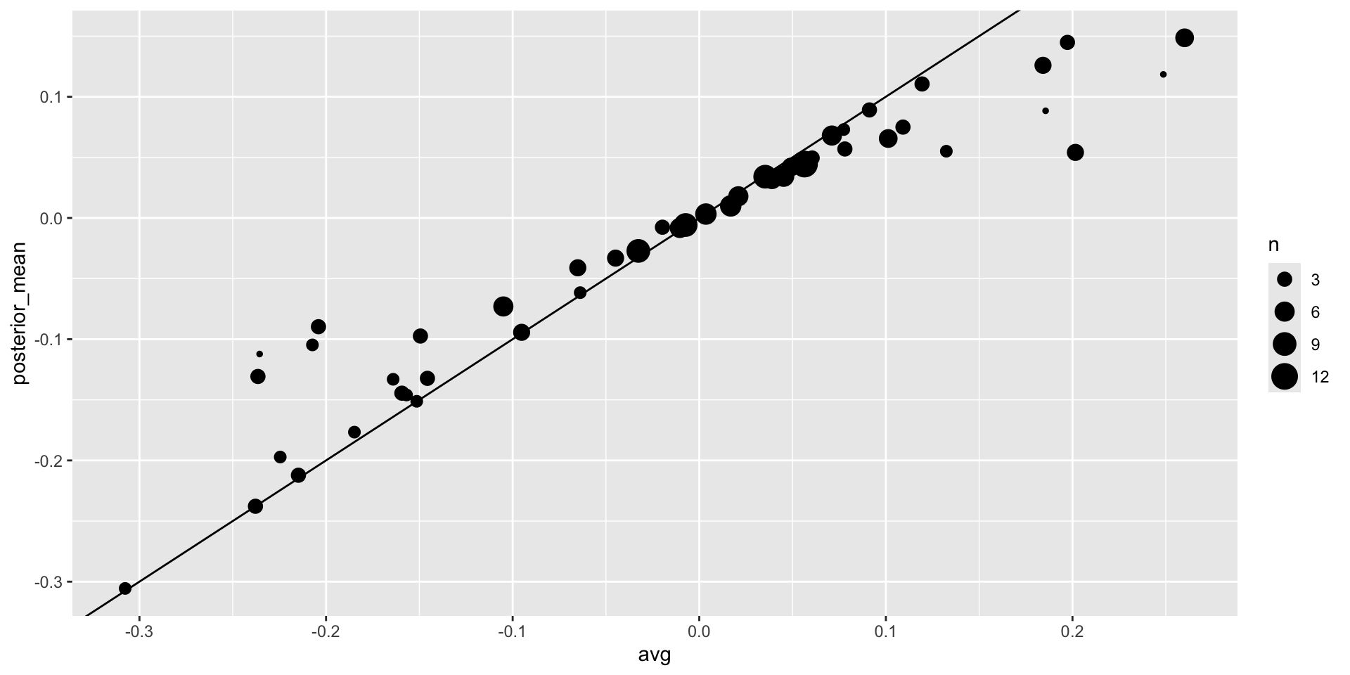
Predicting the electoral college

Now, we repeat this 10,000 times and generate an outcome from the posterior.
In each iteration, we track the total number of electoral votes for Clinton.
Remember that Trump gets 270 votes minus the ones for Clinton.
Also, note that the reason we add 7 in the code is to account for Rhode Island and D.C.

Predicting the electoral college

B <- 10000 
mu <- 0 
tau <- 0.02 
clinton_EV <- replicate(B, { 
  results |> mutate(sigma = sd/sqrt(n),  
                   B = ifelse(n >= 5, sigma^2 / (sigma^2 + tau^2), 0), 
                   posterior_mean = B*mu + (1 - B)*avg, 
                   posterior_se = sqrt(1/(1/sigma^2 + 1/tau^2)), 
                   result = rnorm(length(posterior_mean),  
                                  posterior_mean, posterior_se), 
                   clinton = ifelse(result > 0, electoral_votes, 0)) |>  
    summarize(clinton = sum(clinton)) |>  
    pull(clinton) + 7 
}) 
mean(clinton_EV > 269)

[1] 0.9982

Predicting the electoral college

This model gives Clinton over 99% chance of winning.
A similar prediction was made by the Princeton Election Consortium.
We now know it was quite off.
What happened?
The model above ignores the general bias and assumes the results from different states are independent.
After the election, we realized that the general bias in 2016 was not that big: it was between 2% and 3%.

Predicting the electoral college

But because the election was close in several big states and these states had a large number of polls, pollsters that ignored the general bias greatly underestimated the standard error.
Using the notation we introduced, they assumed the standard error was \(\sqrt{\sigma^2/N}\).
With large \(N\), this estimate is substiantially closer to 0 than the more accurate estimate \(\sqrt{\sigma^2/N + \sigma_b^2}\).
FiveThirtyEight, which models the general bias in a rather sophisticated way, reported a closer result.

Predicting the electoral college

We can simulate the results now with a bias term.
For the state level, the general bias can be larger so we set it at \(\sigma_b = 0.035\):

Predicting the electoral college

tau <- 0.02 
bias_sd <- 0.035 
clinton_EV_2 <- replicate(10000, { 
  results |> mutate(sigma = sd/sqrt(n), 
                    #few polls means not in play so don't shrink 
                    B = ifelse(n >= 5, sigma^2 / (sigma^2 + tau^2), 0), 
                    posterior_mean = B*mu + (1 - B)*avg, 
                    posterior_se = sqrt(1/(1/sigma^2 + 1/tau^2)), 
                    result = rnorm(length(posterior_mean),  
                                  posterior_mean, sqrt(posterior_se^2 + bias_sd^2)), 
                   clinton = ifelse(result > 0, electoral_votes, 0)) |>  
    summarize(clinton = sum(clinton) + 7) |>  
    pull(clinton) 
}) 
mean(clinton_EV_2 > 269)

[1] 0.8878

This gives us a much more sensible estimate.

Predicting the electoral college

Looking at the outcomes of the simulation, we see how the bias term adds variability to the final results.

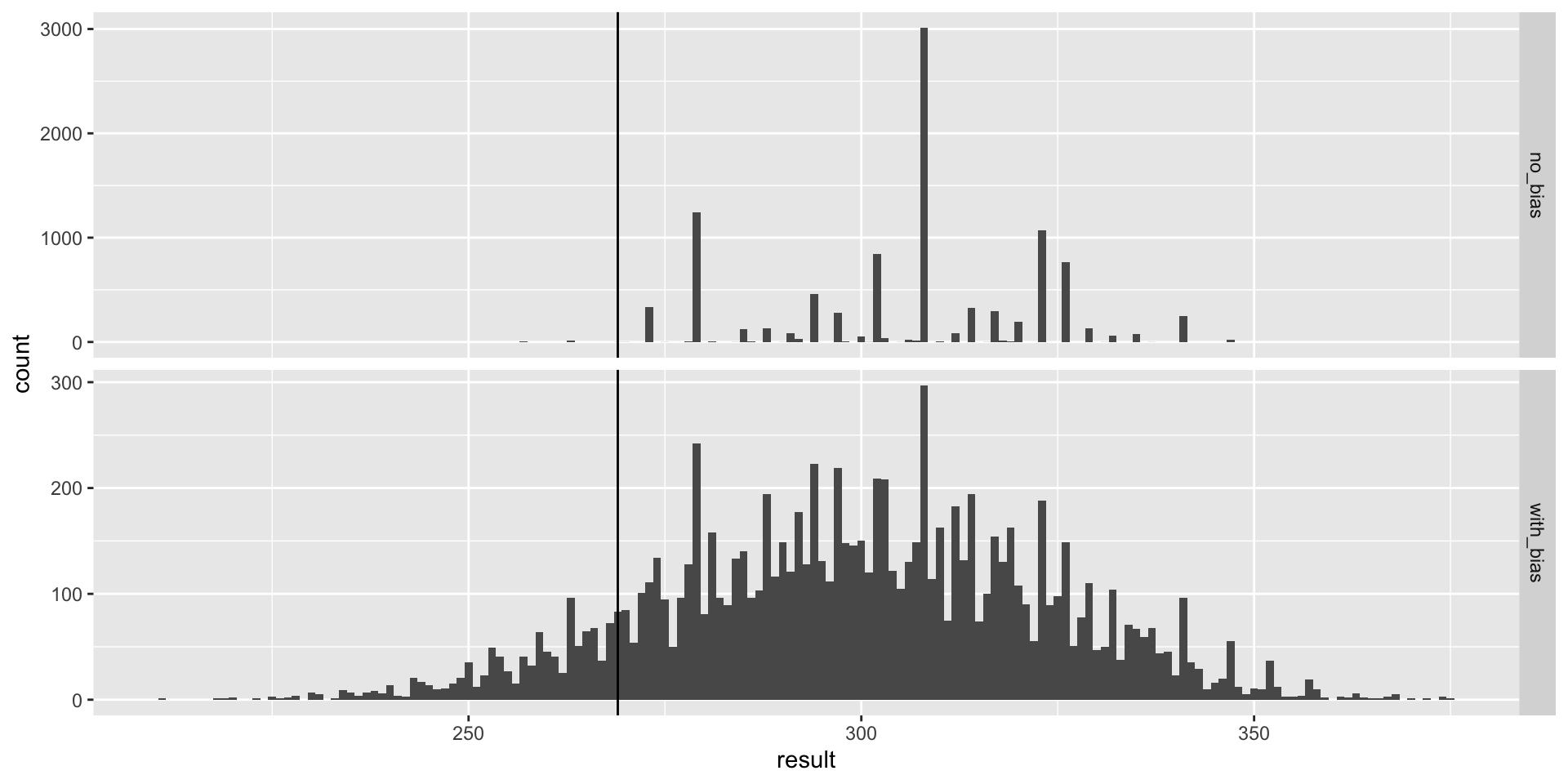
Predicting the electoral college

FiveThirtyEight includes many other features we do not include here.
One is that they model variability with distributions that have high probabilities for extreme events compared to the normal.
One way we could do this is by changing the distribution used in the simulation from a normal distribution to a t-distribution.
FiveThirtyEight predicted a probability of 71%.

Forecasting

Forecasters like to make predictions well before the election.
The predictions are adapted as new poll results are released.
However, an important question forecasters must ask is: How informative are polls taken several weeks before the election about the actual election? Here, we study the variability of poll results across time.

Forecasting

To make sure the variability we observe is not due to pollster effects, let’s study data from one pollster:

one_pollster <- polls_us_election_2016 |>  
  filter(pollster == "Ipsos" & state == "U.S.") |>  
  mutate(spread = rawpoll_clinton/100 - rawpoll_trump/100)

Forecasting

Since there is no pollster effect, then perhaps the theoretical standard error matches the data-derived standard deviation.
We compute both here:

se <- one_pollster |>  
  summarize(empirical = sd(spread),  
            theoretical = 2*sqrt(mean(spread)*(1 - mean(spread))/min(samplesize))) 
se

   empirical theoretical
1 0.04025194  0.03256719

Forecasting

But the empirical standard deviation is higher than the highest possible theoretical estimate. Furthermore, the spread data does not look normal as the theory would predict:

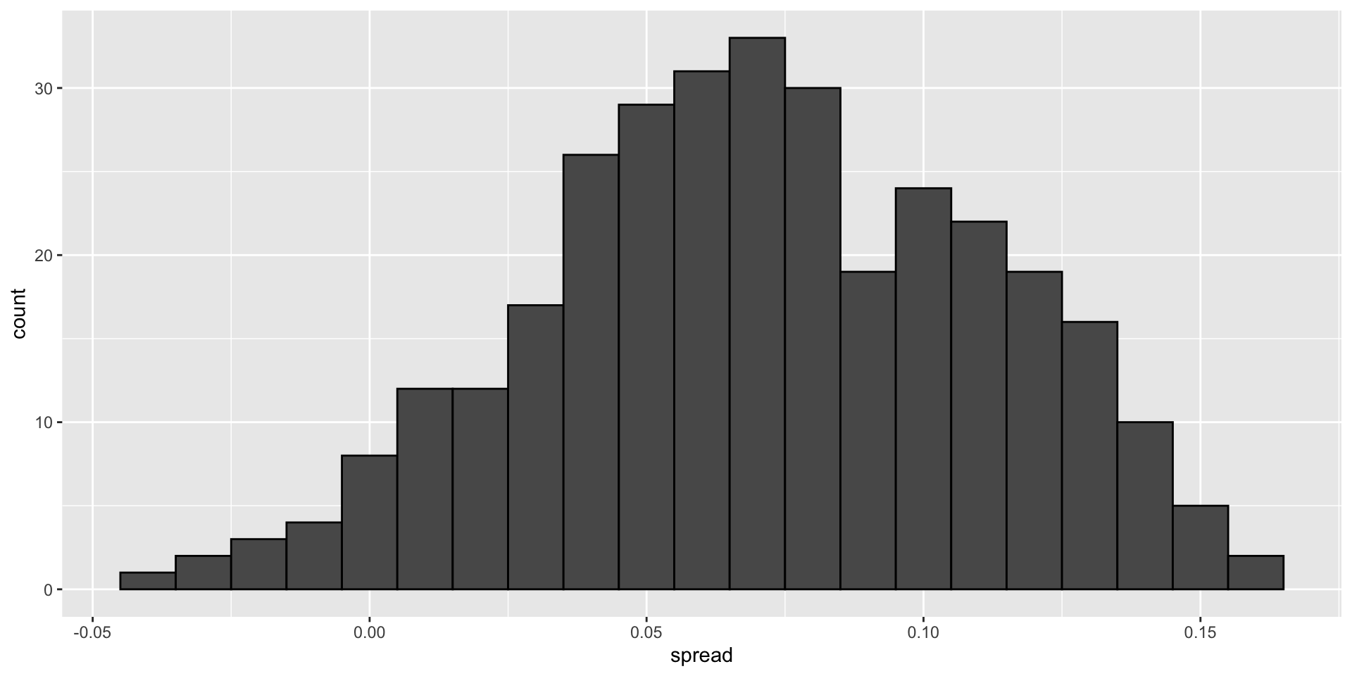
Forecasting

The models we have described include pollster-to-pollster variability and sampling error.
But this plot is for one pollster and the variability we see is certainly not explained by sampling error.
Where is the extra variability coming from?

Forecasting

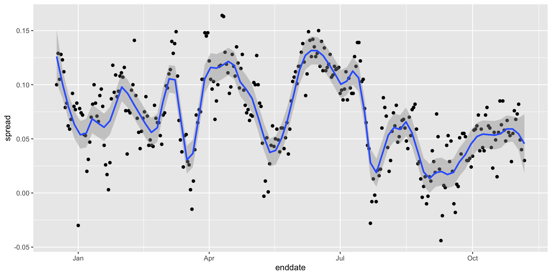
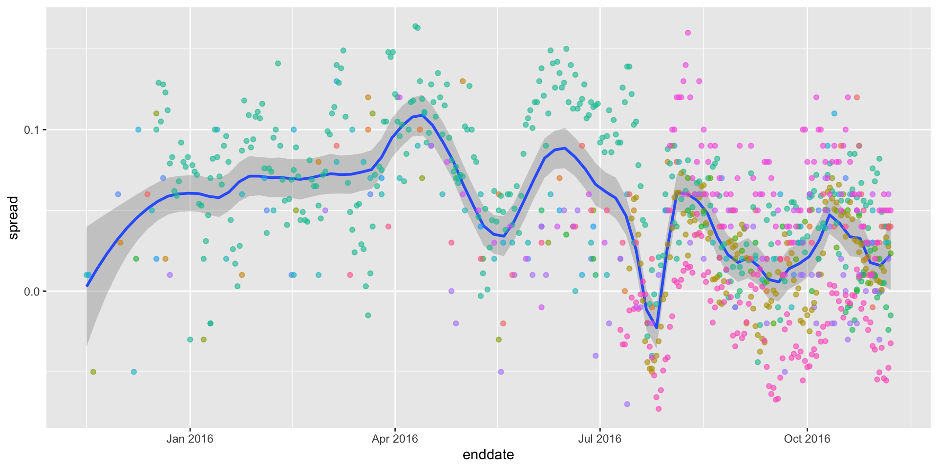
The following plots make a strong case that it comes from time fluctuations not accounted for by the theory that assumes \(p\) is fixed:

Forecasting

Some of the peaks and valleys we see coincide with events such as the party conventions, which tend to give the candidate a boost. We can see that the peaks and valleys are consistent across several pollsters:

Forecasting

This implies that if we are going to forecast, we must include a term to accounts for the time effect.
We can add a bias term for time and denote as \(b_t\).
The standard deviation of \(b_t\) would depend on \(t\) since the closer we get to election day, the closer to 0 this bias term should be.
Pollsters also try to estimate trends from these data and incorporate them into their predictions.
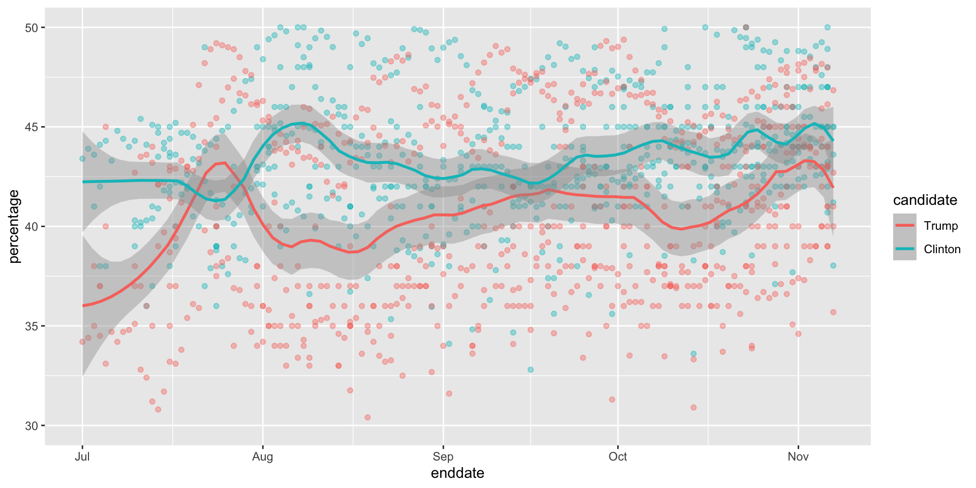
We can model the time trend \(b_t\) with a smooth function.

Forecasting

We usually see the trend estimate not for the difference, but for the actual percentages for each candidate like this: