library(tidyverse)
library(dslabs)
mu <- 0.039
Ns <- c(1298, 533, 1342, 897, 774, 254, 812, 324, 1291, 1056, 2172, 516)
p <- (mu + 1) / 2
polls <- map_df(Ns, function(N) {
  x <- sample(c(0, 1), size = N, replace = TRUE, prob = c(1 - p, p))
  x_hat <- mean(x)
  se_hat <- sqrt(x_hat * (1 - x_hat) / N)
  list(estimate = 2 * x_hat - 1,
    low = 2*(x_hat - 1.96*se_hat) - 1,
    high = 2*(x_hat + 1.96*se_hat) - 1,
    sample_size = N)
}) |>
mutate(poll = seq_along(Ns)) Data-driven models
2024-10-28
Data-driven models
“All models are wrong, but some are useful.” –George E.P. Box.
Data-driven models
Our analysis of poll-related results has been based on a simple sampling model.
This model assumes that each voter has an equal chance of being selected for the poll, similar to picking beads from an urn with two colors.
However, in this section, we explore real-world data and discover that this model is incorrect.
Data-driven models
- However, these introductions are just scratching the surface, and readers interested in statistical modeling should supplement the material presented in this book with additional references.
Case study: poll aggregators
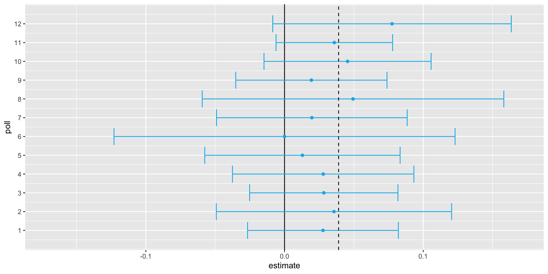
We generate results for 12 polls taken the week before the election.
We mimic sample sizes from actual polls, construct, and report 95% confidence intervals for each of the 12 polls.
We save the results from this simulation in a data frame and add a poll ID column.
Case study: poll aggregators
Case study: poll aggregators
Case study: poll aggregators
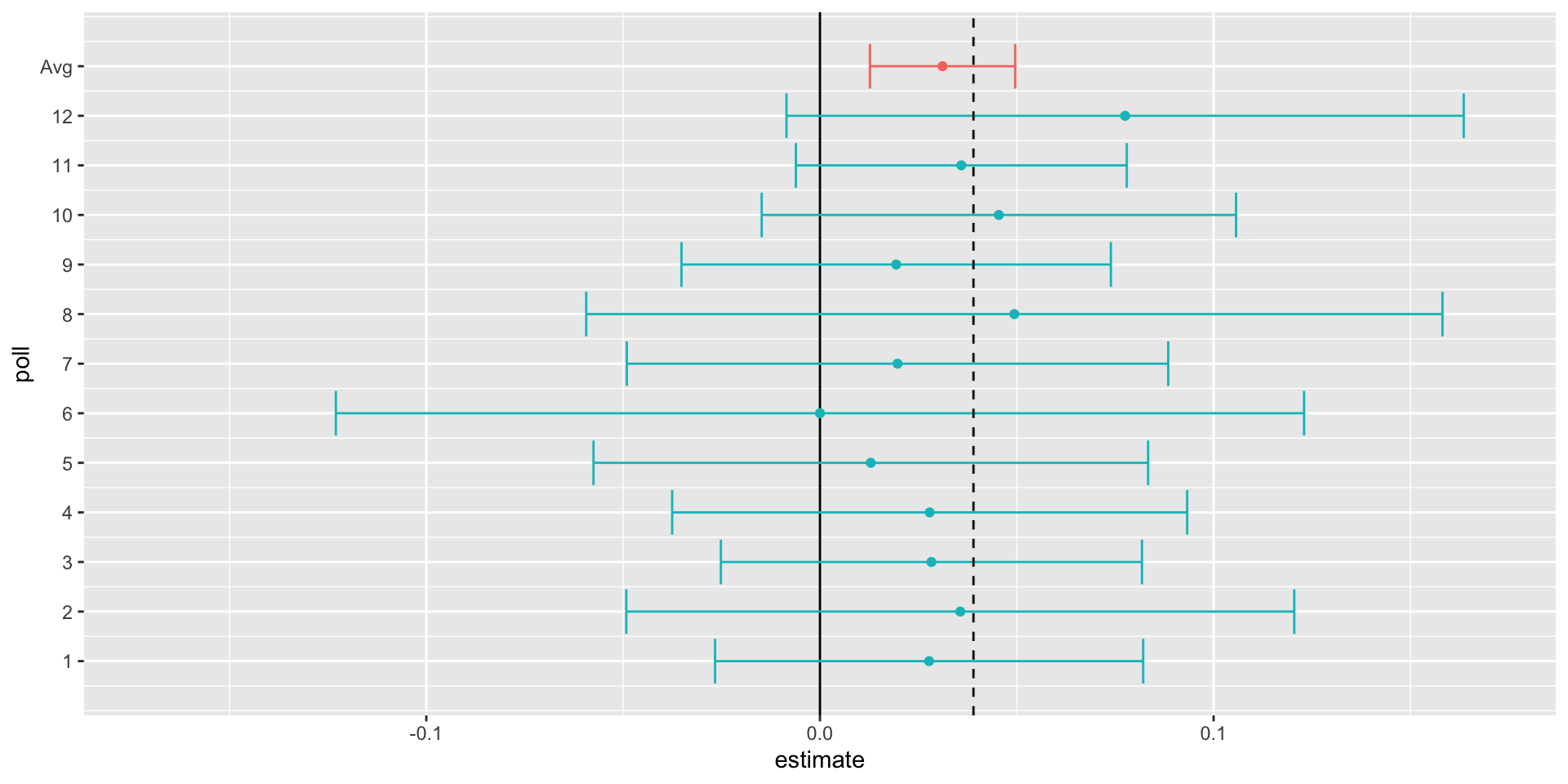
Poll aggregators combine polls to improve power.
By doing this, we are effectively conducting a poll with a huge sample size.
Although, as aggregators, we do not have access to the raw poll data.
We can use math to reconstruct what we would have obtained with one large poll with sample size:
Case study: poll aggregators
- Basically, we construct an estimate of the spread, let’s call it \(\mu\), with a weighted average in the following way:
Case study: poll aggregators
- We can reconstruct the margin of error as well:
[1] 0.01845451- Which is much smaller than any of the individual polls.
Case study: poll aggregators
The aggregator estimate is in red:
Case study: poll aggregators
However, this was just a simulation to illustrate the idea.
Let’s look at real data from the 2016 presidential election.
Case study: poll aggregators
- We add a spread estimate:
Case study: poll aggregators
We are interested in the spread \(2p-1\).
Let’s call the spread \(\mu\) (for difference).
We have 49 estimates of the spread.
The theory we learned from sampling models tells us that these estimates are a random variable with a probability distribution that is approximately normal.
The expected value is the election night spread \(\mu\) and the standard error is \(2\sqrt{p (1 - p) / N}\).
Case study: poll aggregators
- We construct a confidence interval assuming the data is from an urn model:
- and the standard error is:
Case study: poll aggregators
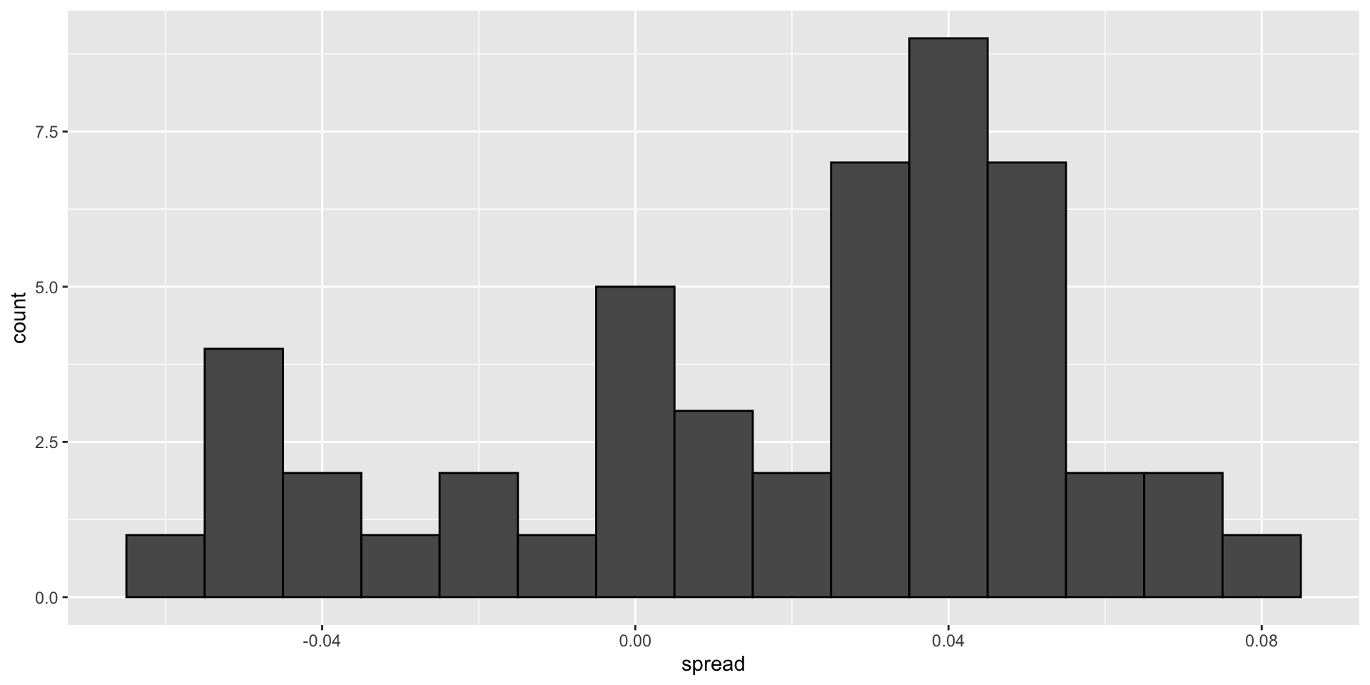
So we report a spread of 1.43% with a margin of error of 0.66%.
On election night, we discover that the actual percentage was 2.1%, which is outside a 95% confidence interval.
What happened?
Case study: poll aggregators
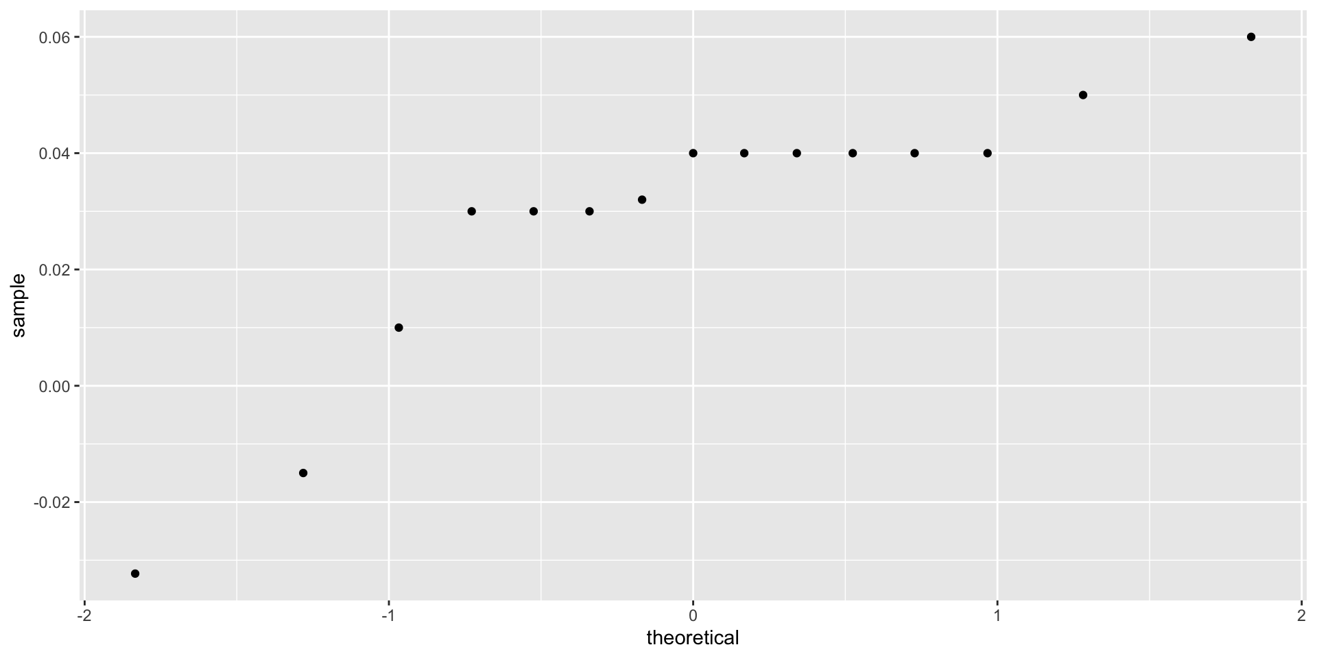
A histogram of the reported spreads reveals a problem:
Case study: poll aggregators
The data does not appear to be normally distributed
The standard error appears to be larger than 0.0066232.
The theory is not working her
This motivates the use of a data-driven model.
Beyond the sampling model
- Data come from various pollsters, some taking several polls:
                                                     pollster n
1                                                    IBD/TIPP 8
2                                    The Times-Picayune/Lucid 8
3                                       USC Dornsife/LA Times 8
4                                    ABC News/Washington Post 7
5                                                       Ipsos 6
6                                     CBS News/New York Times 2
7  Fox News/Anderson Robbins Research/Shaw & Company Research 2
8                                           Angus Reid Global 1
9                                               Insights West 1
10                                             Marist College 1
11                                        Monmouth University 1
12                                            Morning Consult 1
13                               NBC News/Wall Street Journal 1
14                      RKM Research and Communications, Inc. 1
15                                           Selzer & Company 1
Beyond the sampling model
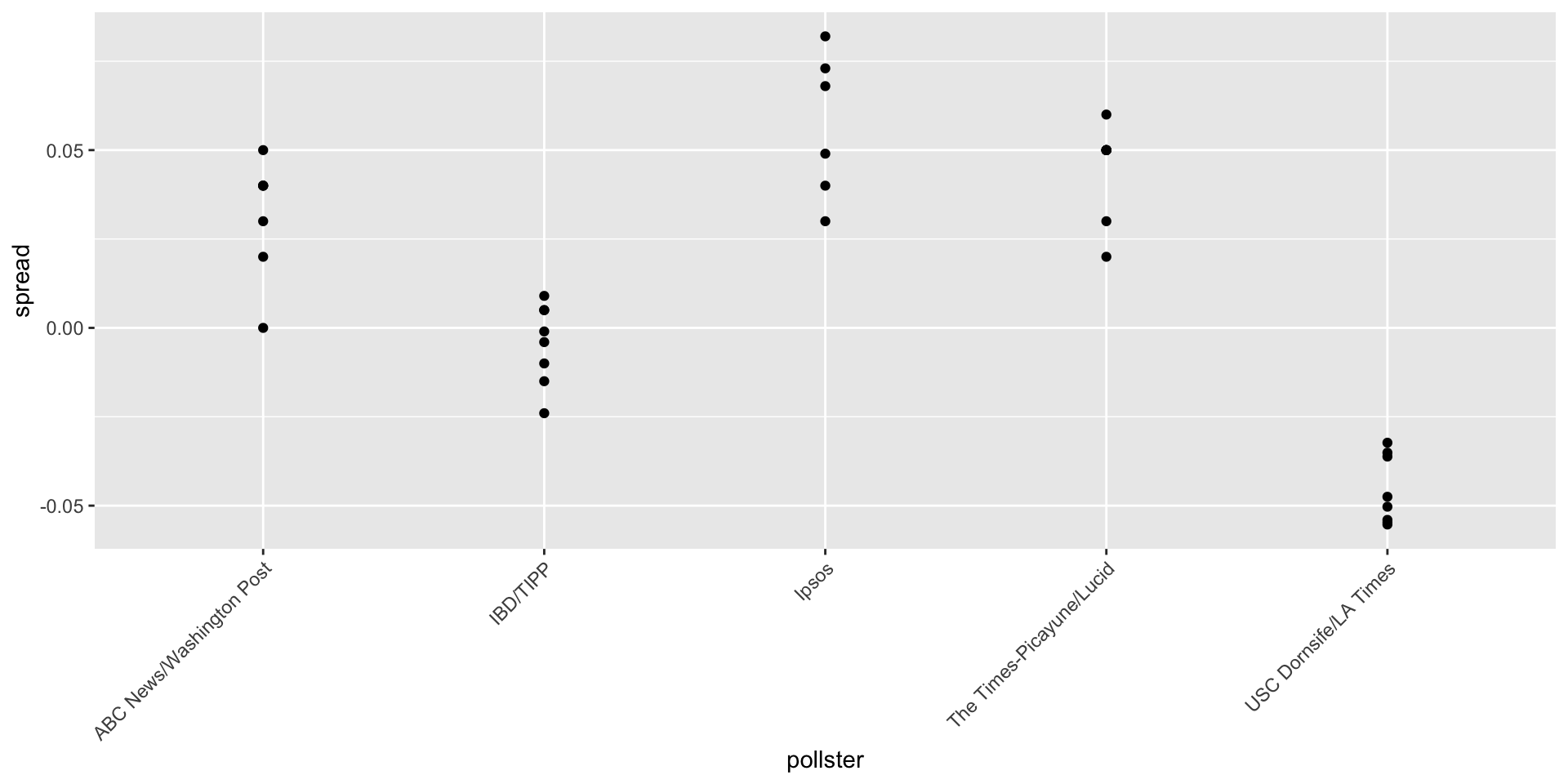
- Let’s visualize the data for the pollsters that are regularly polling:

Beyond the sampling model
This plot reveals an unexpected result.
The standard error predicted by theory is between 0.018 and 0.033:
polls |> group_by(pollster) |>
  filter(n() >= 6) |>
  summarize(se = 2*sqrt(p_hat*(1 - p_hat)/median(samplesize)))
# A tibble: 5 × 2
pollster se
<fct> <dbl>
1 ABC News/Washington Post 0.0265
2 IBD/TIPP 0.0333
3 Ipsos 0.0225
4 The Times-Picayune/Lucid 0.0196
5 USC Dornsife/LA Times 0.0183- This agrees with the within poll variation we see.
Beyond the sampling model
- However, there appears to be differences across the polls:
Beyond the sampling model
Sompling theory says nothing about different pollsters having expected values.
FiveThirtyEight refers to these differences as house effects.
We also call them pollster bias.
Rather than modeling the process generating these values with an urn model, we instead model the pollster results directly.
Beyond the sampling model
To do this, we start by collecting some data.
Specifically, for each pollster, we look at the last reported result before the election:
Beyond the sampling model
- Here is a histogram of the data for these 15 pollsters:
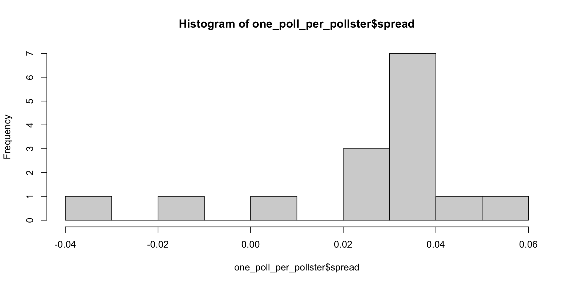
Beyond the sampling model
Although we are no longer using a model with red (Republicans) and blue (Democrats) beads in an urn, our new model can also be thought of as an urn model, but containing poll results from all possible pollsters.
Think of our $N=$15 data points \(X_1,\dots X_N\) as a random sample from this urn.
To develop a useful model, we assume that the expected value of our urn is the actual spread \(\mu=2p-1\), which implies that the sample average has expected value \(\mu\).
Beyond the sampling model
Now, because instead of 0s and 1s, our urn contains continuous numbers, the standard deviation of the urn is no longer \(\sqrt{p(1-p)}\).
Rather than voter sampling variability, the standard error now includes the pollster-to-pollster variability.
Our new urn also includes the sampling variability from the polling.
Regardless, this standard deviation is now an unknown parameter.
Beyond the sampling model
In statistics textbooks, the Greek symbol \(\sigma\) is used to represent this parameter.
So our new statistical model is that \(X_1, \dots, X_N\) are a random sample with expected \(\mu\) and standard deviation \(\sigma\).
The distribution, for now, is unspecified.
Beyond the sampling model
- Assume \(N\) is large enough to assume the sample average \(\bar{X} = \sum_{i=1}^N X_i\) follows a normal distribution with expected value \(\mu\) and standard error \(\sigma / \sqrt{N}\).
\[ \bar{X} \sim \mbox{N}(\mu, \sigma / \sqrt{N}) \]
Here the \(\sim\) symbol tells us that the random variable on the left follows the distribution on the right.
We use the notation \(N(a,b)\) to represent the normal distribution with mean \(a\) and standard deviation \(b\).
Estimating the SD
Our new model has two unknown parameters: the expected value \(\mu\) and the standard deviation \(\sigma\).
We know that the sample average \(\bar{X}\) will be our estimate of \(\mu\).
But what about \(\sigma\)?
Estimating the SD
- Theory tells us that we can estimate the urn model \(\sigma\) with the sample standard deviation defined as:
\[ s = \sqrt{ \frac{1}{N-1} \sum_{i=1}^N (X_i - \bar{X})^2 } \]
Unlike for the population standard deviation definition, we now divide by \(N-1\).
This makes \(s\) a better estimate of \(\sigma\).
There is a mathematical explanation for this, which is explained in most statistics textbooks.
Estimating the SD
- The
sdfunction in R computes the sample standard deviation:
Computing a confidence interval
- We are now ready to form a new confidence interval based on our new data-driven model:
results <- one_poll_per_pollster |>
  summarize(avg = mean(spread),
            se = sd(spread)/sqrt(length(spread))) |>
  mutate(start = avg - 1.96*se,
         end = avg + 1.96*se)
round(results*100, 1)
avg se start end
1 2.9 0.6 1.7 4.1Our confidence interval is wider now since it incorporates the pollster variability.
It does include the election night result of 2.1%.
Also, note that it was small enough not to include 0, which means we were confident Clinton would win the popular vote.
The t-distribution
Above, we made use of the CLT with a sample size of 15.
Because we are estimating a second parameters \(\sigma\), further variability is introduced into our confidence interval, which results in intervals that are too small.
The t-distribution
For very large sample sizes, this extra variability is negligible, but in general, for values smaller than 30, we need to be cautious about using the CLT.
However, if the data in the urn is known to follow a normal distribution, then we actually have mathematical theory that tells us how much bigger we need to make the intervals to account for the estimation of \(\sigma\).
Applying this theory, we can construct confidence intervals for any \(N\).
But again, this works only if the data in the urn is known to follow a normal distribution.
So for the 0, 1 data of our previous urn model, this theory definitely does not apply.
Warning
Note that 30 is a very general rule of thumb based on the case when the data come from a normal distribution.
There are cases when a large sample size is needed as well as cases when smaller sample sizes are good enough.
The t-distribution
- The statistic on which confidence intervals for \(\mu\) are based is:
\[ Z = \frac{\bar{X} - \mu}{\sigma/\sqrt{N}} \]
- CLT tells us that Z is approximately normally distributed with expected value 0 and standard error 1.
The t-distribution
- But in practice we don’t know \(\sigma\), so we use:
\[ t = \frac{\bar{X} - \mu}{s/\sqrt{N}} \]
- This is referred to as a t-statistic.
The t-distribution
By substituting \(\sigma\) with \(s\), we introduce some variability.
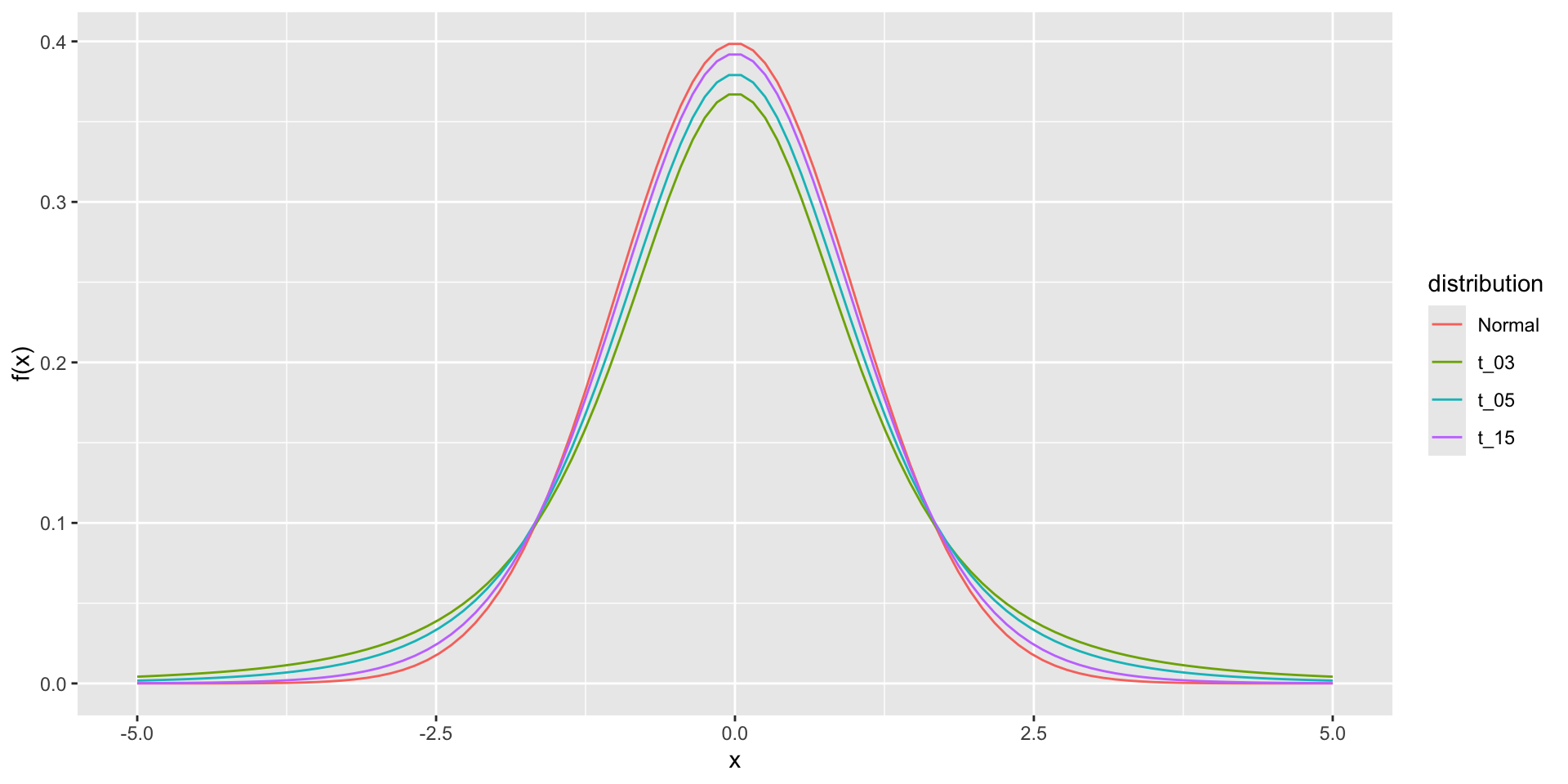
Theory tells us that \(t\) follows a student t-distribution with \(N-1\) degrees of freedom (df).
The df is a parameter that controls the variability via fatter tails:
The t-distribution
- If we are willing to assume the pollster effect data is normally distributed, based on the sample data \(X_1, \dots, X_N\),
The t-distribution
- then \(t\) follows a t-distribution with \(N-1\) degrees of freedom.
The t-distribution
- So perhaps a better confidence interval for \(\mu\) is:
z <- qt(0.975,  nrow(one_poll_per_pollster) - 1)
one_poll_per_pollster |>
  summarize(avg = mean(spread), moe = z*sd(spread)/sqrt(length(spread))) |>
  mutate(start = avg - moe, end = avg + moe)
# A tibble: 1 × 4
avg moe start end
<dbl> <dbl> <dbl> <dbl>
1 0.0290 0.0134 0.0156 0.0424- A bit larger than the one using normal is:
The t-distribution
- This results in a slightly larger confidence interval than we obtained before:
  start end
1   1.6 4.2
The t-distribution
Note that using the t-distribution and the t-statistic is the basis for t-tests, a widely used approach for computing p-values.
To learn more about t-tests, you can consult any statistics textbook.
The t-distribution can also be used to model errors in bigger deviations that are more likely than with the normal distribution, as seen in the densities we previously observed.
FiveThirtyEight uses the t-distribution to generate errors that better model the deviations we see in election data.
The t-distribution
For example, in Wisconsin, the average of six polls was 7% in favor of Clinton with a standard deviation of 1%, but Trump won by 0.7%.
Even after taking into account the overall bias, this 7.7% residual is more in line with t-distributed data than the normal distribution.
The t-distribution
polls_us_election_2016 |>
  filter(state == "Wisconsin" &
           enddate >= "2016-10-31" &
           (grade %in% c("A+", "A", "A-", "B+") | is.na(grade))) |>
  mutate(spread = rawpoll_clinton/100 - rawpoll_trump/100) |>
  mutate(state = as.character(state)) |>
  left_join(results_us_election_2016, by = "state") |>
  mutate(actual = clinton/100 - trump/100) |>
  summarize(actual = first(actual), avg = mean(spread),
            sd = sd(spread), n = n()) |>
  select(actual, avg, sd, n)
actual avg sd n
1 -0.007 0.07106667 0.01041454 6