Confidence Intervals
2024-10-23
Confidence intervals
Confidence intervals are a very useful concept widely employed by data analysts.
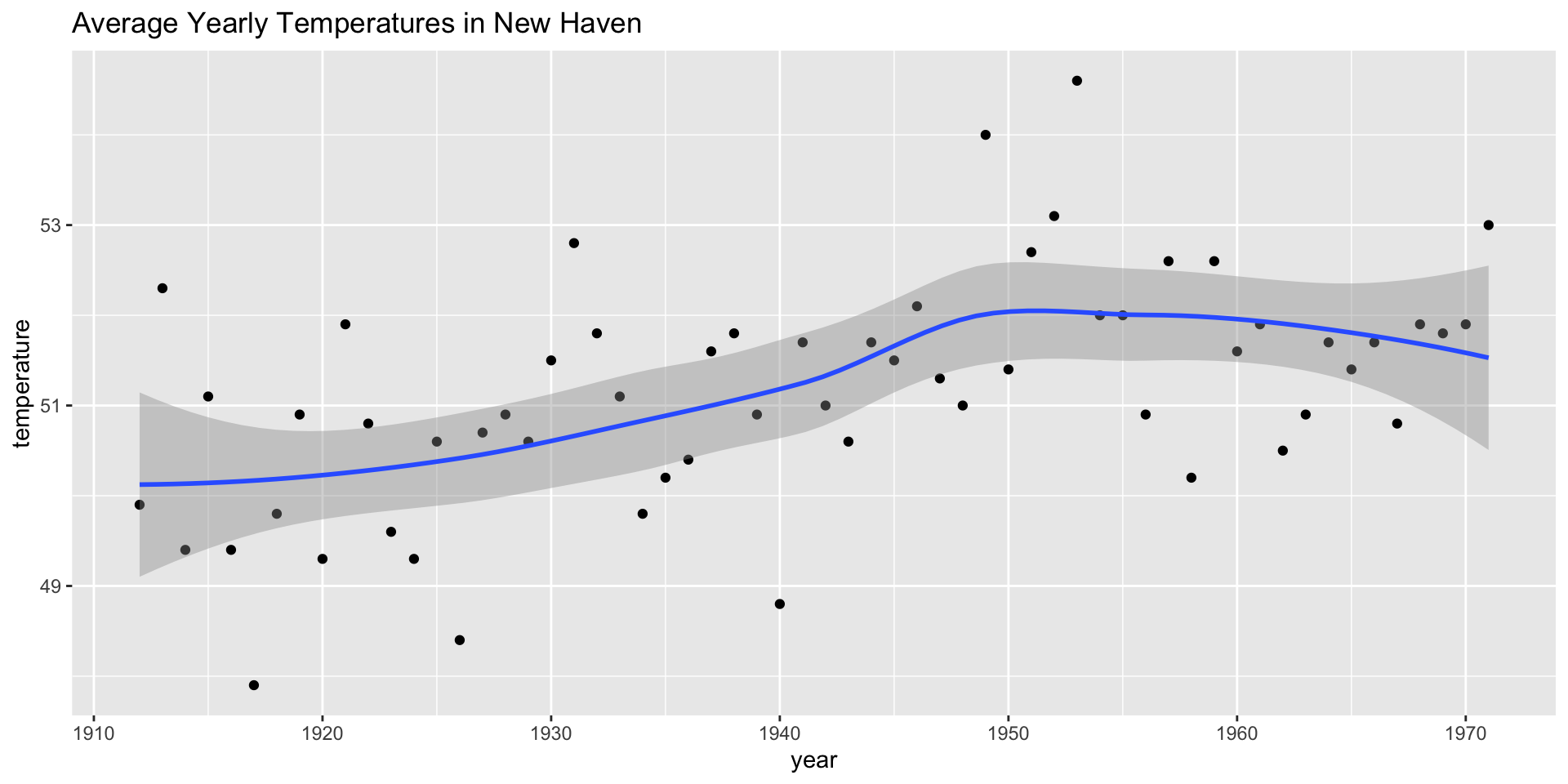
A version of these that are commonly seen come from the
ggplotgeometrygeom_smooth.Below is an example using a temperature dataset available in R:
Confidence intervals
Confidence intervals
In our competition, you were asked to give an interval.
If the interval you submitted includes the \(p\), you receive half the money you spent on your “poll” back and proceed to the next stage of the competition.
Confidence intervals
One way to pass to the second round is to report a very large interval.
For example, the interval \([0,1]\) is guaranteed to include \(p\).
However, with an interval this big, we have no chance of winning the competition.
Confidence intervals
Similarly, if you are an election forecaster and predict the spread will be between -100% and 100%, you will be ridiculed for stating the obvious.
Even a smaller interval, such as saying the spread will be between -10 and 10%, will not be considered serious.
Confidence intervals
On the other hand, the smaller the interval we report, the smaller our chances are of winning the prize.
Likewise, a bold pollster that reports very small intervals and misses the mark most of the time will not be considered a good pollster.
We might want to be somewhere in between.
We can use the statistical theory we have learned to compute the probability of any given interval including \(p\).
Confidence intervals
To illustrate this we run the Monte Carlo simulation.
We use the same parameters as above:
Confidence intervals
- And notice that the interval here:
x <- sample(c(0, 1), size = N, replace = TRUE, prob = c(1 - p, p))
x_hat <- mean(x)
se_hat <- sqrt(x_hat*(1 - x_hat)/N)
c(x_hat - 1.96*se_hat, x_hat + 1.96*se_hat)
[1] 0.4032809 0.4647191- is different from this one:
x <- sample(c(0,1), size = N, replace = TRUE, prob = c(1 - p, p))
x_hat <- mean(x)
se_hat <- sqrt(x_hat*(1 - x_hat)/N)
c(x_hat - 1.96*se_hat, x_hat + 1.96*se_hat)
[1] 0.4301041 0.4918959- Keep sampling and creating intervals, and you will see the random variation.
Confidence intervals
- To determine the probability that the interval includes \(p\), we need to compute the following:
\[ \mbox{Pr}\left(\bar{X} - 1.96\hat{\mbox{SE}}(\bar{X}) \leq p \leq \bar{X} + 1.96\hat{\mbox{SE}}(\bar{X})\right) \]
Confidence intervals
- By subtracting and dividing the same quantities in all parts of the equation, we find that the above is equivalent to:
\[ \mbox{Pr}\left(-1.96 \leq \frac{\bar{X}- p}{\hat{\mbox{SE}}(\bar{X})} \leq 1.96\right) \]
Confidence intervals
- The term in the middle is an approximately normal random variable with expected value 0 and standard error 1, which we have been denoting with \(Z\), so we have:
\[ \mbox{Pr}\left(-1.96 \leq Z \leq 1.96\right) \]
- which we can quickly compute using :
- proving that we have a 95% probability.
Confidence intervals
- If we want to have a larger probability, say 99%, we need to multiply by whatever
zsatisfies the following:
\[ \mbox{Pr}\left(-z \leq Z \leq z\right) = 0.99 \]
- We use:
Confidence intervals
In statistics textbooks, confidence interval formulas are given for arbitraty probabilities written as \(1-\alpha\).
We can obtain the \(z\) for the equation above using
z = qnorm(1 - alpha / 2)because \(1 - \alpha/2 - \alpha/2 = 1 - \alpha\).So, for example, for \(\alpha=0.05\), \(1 - \alpha/2 = 0.975\) and we get the \(z=1.96\) we used above:
A Monte Carlo simulation
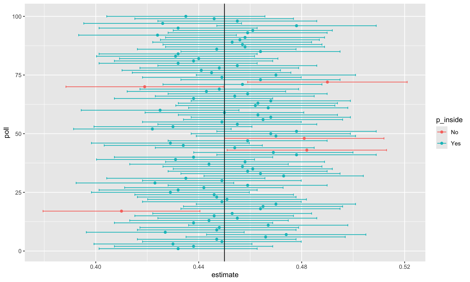
- We can run a Monte Carlo simulation to confirm that, in fact, a 95% confidence interval includes \(p\) 95% of the time.
A Monte Carlo simulation
- The following plot shows the first 100 confidence intervals.