Parameters and Estimates

2024-10-23

The sampling model for polls

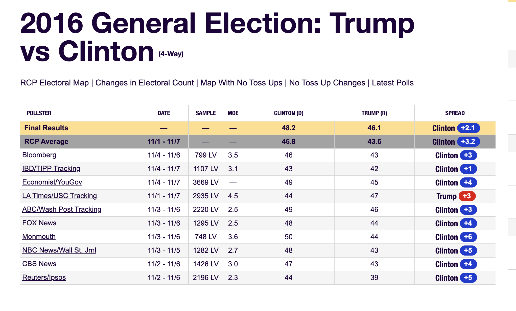
The week before the election Real Clear Politics showed this:

The sampling model for polls

To help us understand the connection between polls and what we have learned, let’s construct a situation similar to what pollsters face.
To simulate the challenge pollsters encounter in terms of competing with other pollsters for media attention, we will use an urn filled with beads to represent voters, and pretend we are competing for a $25 dollar prize.
The challenge is to guess the spread between the proportion of blue and red beads in an urn.

The sampling model for polls

Before making a prediction, you can take a sample (with replacement) from the urn.
To reflect the fact that running polls is expensive, it costs you $0.10 for each bead you sample.
Therefore, if your sample size is 250, and you win, you will break even since you would have paid $25 to collect your $25 prize.
Your entry into the competition can be an interval.

The sampling model for polls

If the interval you submit contains the true proportion, you receive half what you paid and proceed to the second phase of the competition.
In the second phase, the entry with the smallest interval is selected as the winner.
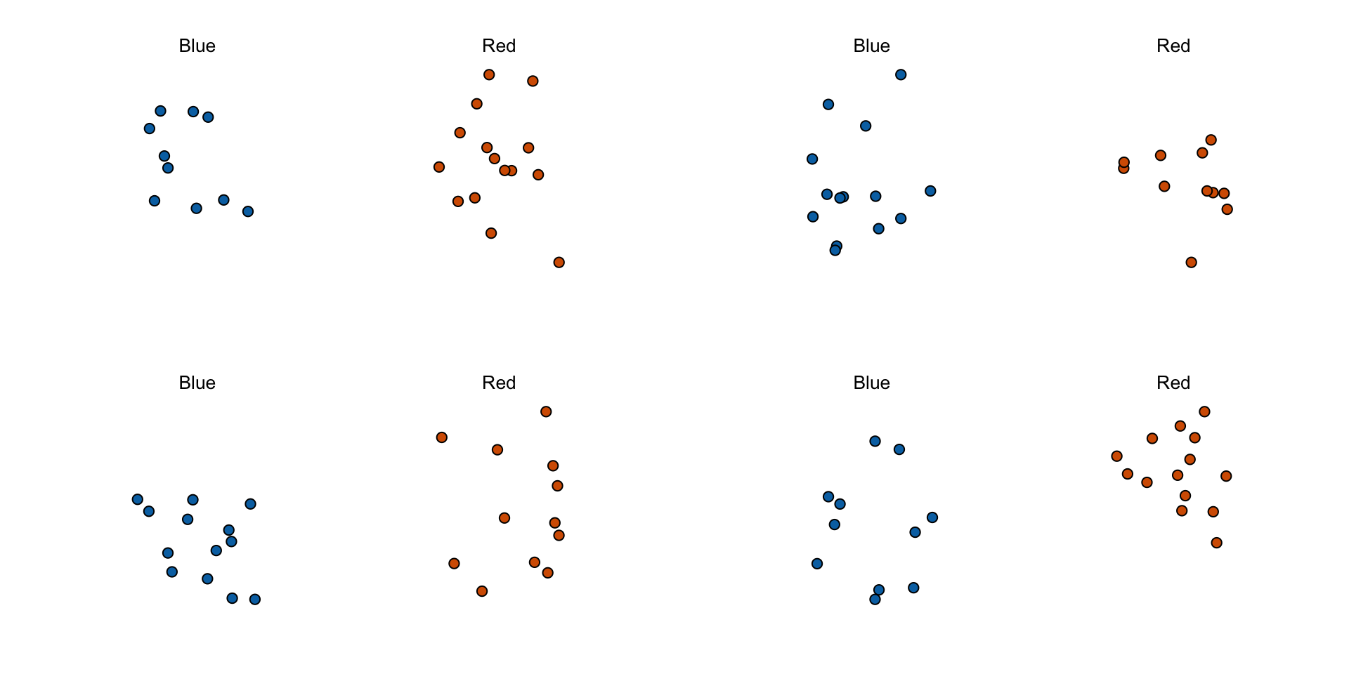
The dslabs package includes a function that shows a random draw from this urn:

set.seed(1)
library(tidyverse) 
library(dslabs) 
take_poll(25)

Populations, samples, parameters, and estimates

We want to predict difference proportion of blue beads - proportion of red beads
Let’s the proportion of blue $p$
We want to estimate $p - (1-p)$ = $2p - 1$.

Populations, samples, parameters, and estimates

In statistical class, the beads in the urn are called the population.
The proportion of blue beads in the population $p$ is called a parameter.
The 25 beads we see in the previous plot are called a sample.

Populations, samples, parameters, and estimates

The goal of statistical inference is to predict the parameter $p$ based on the observed data in the sample.
Can we do this with the 25 observations above? It is certainly informative.
For example, given that we see 13 red and 12 blue beads, it is unlikely that $p$ > .9 or $p$ < .1.
We want to construct an estimate of $p$ using only the information we observe.

Populations, samples, parameters, and estimates

Observe that in the four random samples shown above, the sample proportions range from 0.44 to 0.60.

The sample average

We use the symbol $\bar{X}$ to represent this average.
In statistics textbooks, a bar on top of a symbol typically denotes the average.
The theory we just covered about the sum of draws becomes useful because the average is a sum of draws multiplied by the constant $1/N$:

\[\bar{X} = \frac{1}{N} \sum_{i=1}^N X_i\]

The sample average

What do we know about the distribution of the sum?
We know that the expected value of the sum of draws is $N$ times the average of the values in the urn.
We know that the average of the 0s and 1s in the urn must be $p$, the proportion of blue beads.
There is an important difference compared to what we did previously: we don’t know the composition of the urn.
This is what we want to find out: we are trying to estimate $p$.

Parameters

Just as we use variables to define unknowns in systems of equations, in statistical inference, we define parameters to represent unknown parts of our models.
We define the parameters $p$ to represent the the proportion of blue beads in the urn.
Since our main goal is determining $p$, we are going to estimate this parameter.
The concepts presented here on how we estimate parameters, and provide insights into how good these estimates are, extend to many data analysis tasks.

Parameters

For example, we may want to determine
- the difference in health improvement between patients receiving treatment and a control group,
- investigate the health effects of smoking on a population,
- analyze the differences in racial groups of fatal shootings by police, or
- assess the rate of change in life expectancy in the US during the last 10 years.

Parameters

All these questions can be framed as a task of estimating a parameter from a sample.
The properties we learned tell us that:

\[ \mbox{E}(\bar{X}) = p \]

and

\[ \mbox{SE}(\bar{X}) = \sqrt{p(1-p)/N} \]

Properties of our estimate

The law of large numbers tells us that with a large enough poll, our estimate converges to $p$.
If we take a large enough poll to make our standard error about 1%, we will be quite certain about who will win.
But how large does the poll have to be for the standard error to be this small?
One problem is that we do not know $p$, so we can’t compute the standard error.

Properties of our estimate

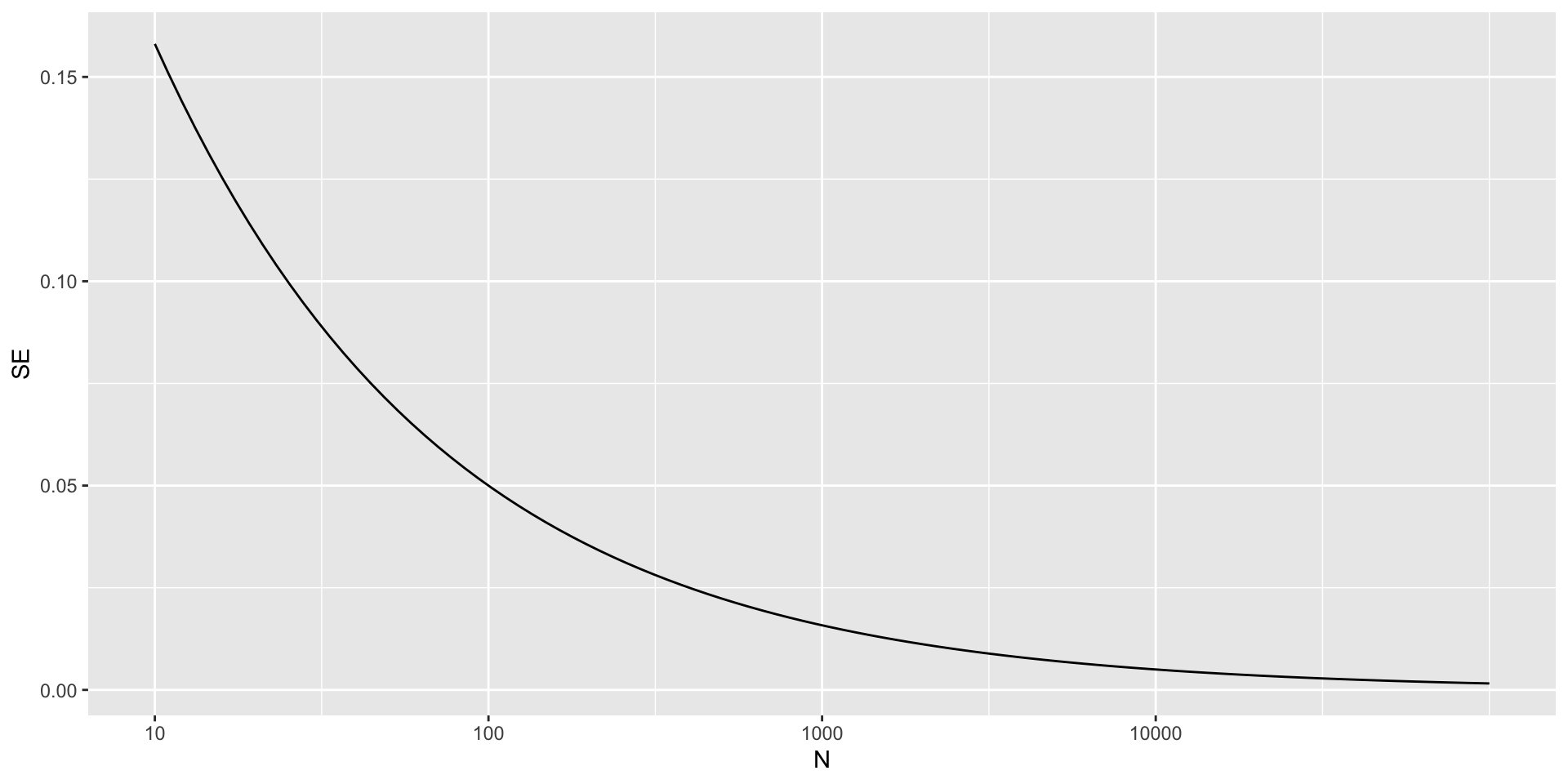
For illustrative purposes, let’s assume that $p=0.51$ and make a plot of the standard error versus the sample size $N$:

Properties of our estimate

The plot shows that we would need a poll of over 10,000 people to achieve a standard error that low.
We rarely see polls of this size due in part to the associated costs.
According to the Real Clear Politics table, sample sizes in opinion polls range from 500-3,500 people.
For a sample size of 1,000 and $p=0.51$, the standard error is:

sqrt(p*(1 - p))/sqrt(1000)

[1] 0.01580823

Properties of our estimate

The CLT tells us that the distribution function for a sum of draws is approximately normal.
Using the properties we learned: $\bar{X}$ has an approximately normal distribution with expected value $p$ and standard error $\sqrt{p(1-p)/N}$.

Central Limit Theorem

Now how can answer questions like what is the probability that we are within 1% from $p$.
We are basically asking what is:

\[ \mbox{Pr}(| \bar{X} - p| \leq .01) \]

which is the same as:

\[ \mbox{Pr}(\bar{X}\leq p + .01) - \mbox{Pr}(\bar{X} \leq p - .01) \]

Central Limit Theorem

Since $p$ is the expected value and $\mbox{SE}(\bar{X}) = \sqrt{p(1-p)/N}$ is the standard error, we get:

\[ \mbox{Pr}\left(Z \leq \frac{ \,.01} {\mbox{SE}(\bar{X})} \right) - \mbox{Pr}\left(Z \leq - \frac{ \,.01} {\mbox{SE}(\bar{X})} \right) \]

Central Limit Theorem

One problem we have is that since we don’t know $p$, we don’t know $\mbox{SE}(\bar{X})$.
However, it turns out that the CLT still works if we estimate the standard error by using $\bar{X}$ in place of $p$.
We say that we plug-in the estimate.
Our estimate of the standard error is therefore:

\[ \hat{\mbox{SE}}(\bar{X})=\sqrt{\bar{X}(1-\bar{X})/N} \]

Central Limit Theorem

Now we continue with our calculation, but dividing by

\[\hat{\mbox{SE}}(\bar{X})=\sqrt{\bar{X}(1-\bar{X})/N})\]

Central Limit Theorem

In our first sample, we had 12 blue and 13 red, so $\bar{X} = 0.48$ and our estimate of standard error is:

x_hat <- 0.48 
se <- sqrt(x_hat*(1-x_hat)/25) 
se

[1] 0.09991997

Central Limit Theorem

Now, we can answer the question of the probability of being close to $p$.
The answer is:

pnorm(0.01/se) - pnorm(-0.01/se)

[1] 0.07971926

Therefore, there is a small chance that we will be close.

Central Limit Theorem

Earlier, we mentioned the margin of error.
Now, we can define it simply as two times the standard error, which we can now estimate.

1.96*se

[1] 0.1958431

Central Limit Theorem

Why do we multiply by 1.96?
Because if you ask what is the probability that we are within 1.96 standard errors from $p$, we get:

\[ \mbox{Pr}\left(Z \leq \, 1.96\,\mbox{SE}(\bar{X}) / \mbox{SE}(\bar{X}) \right) - \mbox{Pr}\left(Z \leq - 1.96\, \mbox{SE}(\bar{X}) / \mbox{SE}(\bar{X}) \right) \]

which is:

\[ \mbox{Pr}\left(Z \leq 1.96 \right) - \mbox{Pr}\left(Z \leq - 1.96\right) = 0.95 \]

Central Limit Theorem

Too see this:

pnorm(1.96) - pnorm(-1.96)

[1] 0.9500042

Central Limit Theorem

There is a 95% probability that $\bar{X}$ will be within $1.96\times \hat{SE}(\bar{X})$, in our case within about 0.2, of $p$.
Observe that 95% is somewhat of an arbitrary choice and sometimes other percentages are used, but it is the most commonly used value to define margin of error.

A Monte Carlo simulation

B <- 10000 
N <- 1000 
x_hat <- replicate(B, { 
  x <- sample(c(0,1), size = N, replace = TRUE, prob = c(1 - p, p)) 
  mean(x) 
})

The problem is, of course, that we don’t know p.

A Monte Carlo simulation

Let’s set p=0.45.
We can then simulate a poll:

p <- 0.45 
N <- 1000 
x <- sample(c(0, 1), size = N, replace = TRUE, prob = c(1 - p, p)) 
x_hat <- mean(x)

In this particular sample, our estimate is x_hat.
We can use that code to do a Monte Carlo simulation:

A Monte Carlo simulation

B <- 10000 
x_hat <- replicate(B, { 
  x <- sample(c(0, 1), size = N, replace = TRUE, prob = c(1 - p, p)) 
  mean(x) 
})

A Monte Carlo simulation

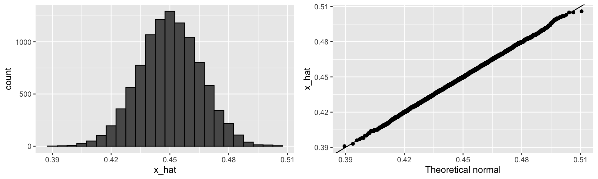
To review, the theory tells us that $\bar{X}$ is approximately normally distributed, has expected value $p=$ 0.45, and standard error $\sqrt{p(1-p)/N}$ = 0.0157321.
The simulation confirms this:

mean(x_hat)

[1] 0.4499836

sd(x_hat)

[1] 0.01556674

A Monte Carlo simulation

A histogram and qqplot confirm that the normal approximation is also accurate:

A Monte Carlo simulation

Of course, in real life, we would never be able to run such an experiment because we don’t know $p$.
However, we can run it for various values of $p$ and $N$ and see that the theory does indeed work well for most values.
You can easily do this by rerunning the code above after changing the values of p and N.

The spread

We did all this theory for the estimate of $p$. How do we estimate the spread $2p - 1$?

Why not run a very large poll?

For realistic values of $p$, let’s say ranging from 0.35 to 0.65, if we conduct a very large poll with 100,000 people, theory tells us that we would predict the election perfectly, as the largest possible margin of error is around 0.3%.

Why not run a very large poll?

One reason is that conducting such a poll is very expensive.
Another, and possibly more important reason, is that theory has its limitations.
Polling is much more complicated than simply picking beads from an urn.
Some people might lie to pollsters, and others might not have phones.

Bias: Why not run a very large poll?

However, perhaps the most important way an actual poll differs from an urn model is that we don’t actually know for sure who is in our population and who is not.
How do we know who is going to vote? Are we reaching all possible voters? Hence, even if our margin of error is very small, it might not be exactly right that our expected value is $p$.
We call this bias.

Bias: Why not run a very large poll?

Historically, we observe that polls are indeed biased, although not by a substantial amount.
The typical bias appears to be about 2-3%.