Matrices In R
2024-11-12
Matrices in R
When the number of variables is large and they can all be represented as a number, it is convenient to store them in a matrix and perform the analysis with linear algebra operations, rather than using tidyverse with data frames.
Variables for each observation are stored in a row, resulting in a matrix with as many columns as variables.
We refer to values represented in the rows of the matrix as the covariates or predictors and, in machine learning, we refer to them as the features.
Matrices in R
In linear algebra, we have three types of objects: scalars, vectors, and matrices.
We have already learned about vectors in R, and, although there is no data type for scalars, we can represent them as vectors of length 1.
Today we learn how to work with matrices in R and relate them to linear algebra notation and concepts.
Case study: MNIST
- The first step in handling mail received in the post office is to sort letters by zip code:
Case study: MNIST
Soon we will describe how we can build computer algorithms to read handwritten digits, which robots then use to sort the letters.
To do this, we first need to collect data, which in this case is a high-dimensional dataset and best stored in a matrix.
Case study: MNIST
- The MNIST dataset was generated by digitizing thousands of handwritten digits, already read and annotated by humans: http://yann.lecun.com/exdb/mnist/
Case study: MNIST
Examples:

Case study: MNIST
- The images are converted into \(28 \times 28 = 784\) pixels:

Case study: MNIST
For each digitized image, indexed by \(i\), we are provided with 784 variables and a categorical outcome, or label, representing the digit among \(0, 1, 2, 3, 4, 5, 6, 7 , 8,\) and \(9\) that the image is representing.
Let’s load the data using the dslabs package:
Case study: MNIST
- In these cases, the pixel intensities are saved in a matrix:
- The labels associated with each image are included in a vector:
Motivating tasks
Visualize the original image. The pixel intensities are provided as rows in a matrix.
Do some digits require more ink to write than others?
Are some pixels uninformative?
Can we remove smudges?
Binarize the data.
Standardize the digits.
Motivating tasks
The tidyverse or data.table are not developed to perform these types of mathematical operations.
For this task, it is convenient to use matrices.
To simplify the code below, we will rename these
xandyrespectively:
Dimensions of a matrix
- The
nrowfunction tells us how many rows that matrix has:
and ncol tells us how many columns:
Dimensions of a matrix
We learn that our dataset contains 60,000 observations (images) and 784 features (pixels).
The
dimfunction returns the rows and columns:
Creating a matrix
- We saw that we can create a matrix using the
matrixfunction.
- Note that by default the matrix is filled in column by column:
Creating a matrix
- To fill the matrix row by row, we can use the
byrowargument:
Creating a matrix
- The function
as.vectorconverts a matrix back into a vector:
Warning
If the product of columns and rows does not match the length of the vector provided in the first argument,
matrixrecycles values.If the length of the vector is a sub-multiple or multiple of the number of rows, this happens without warning:
Subsetting
- To extract a specific entry from a matrix, for example the 300th row of the 100th column, we write:
Subsetting
We can extract subsets of the matrices by using vectors of indexes.
For example, we can extract the first 100 pixels from the first 300 observations like this:
Subsetting
- To extract an entire row or subset of rows, we leave the column dimension blank.
Subsetting
Similarly, we can subset any number of columns by keeping the first dimension blank.
Here is the code to extract the first 100 pixels:
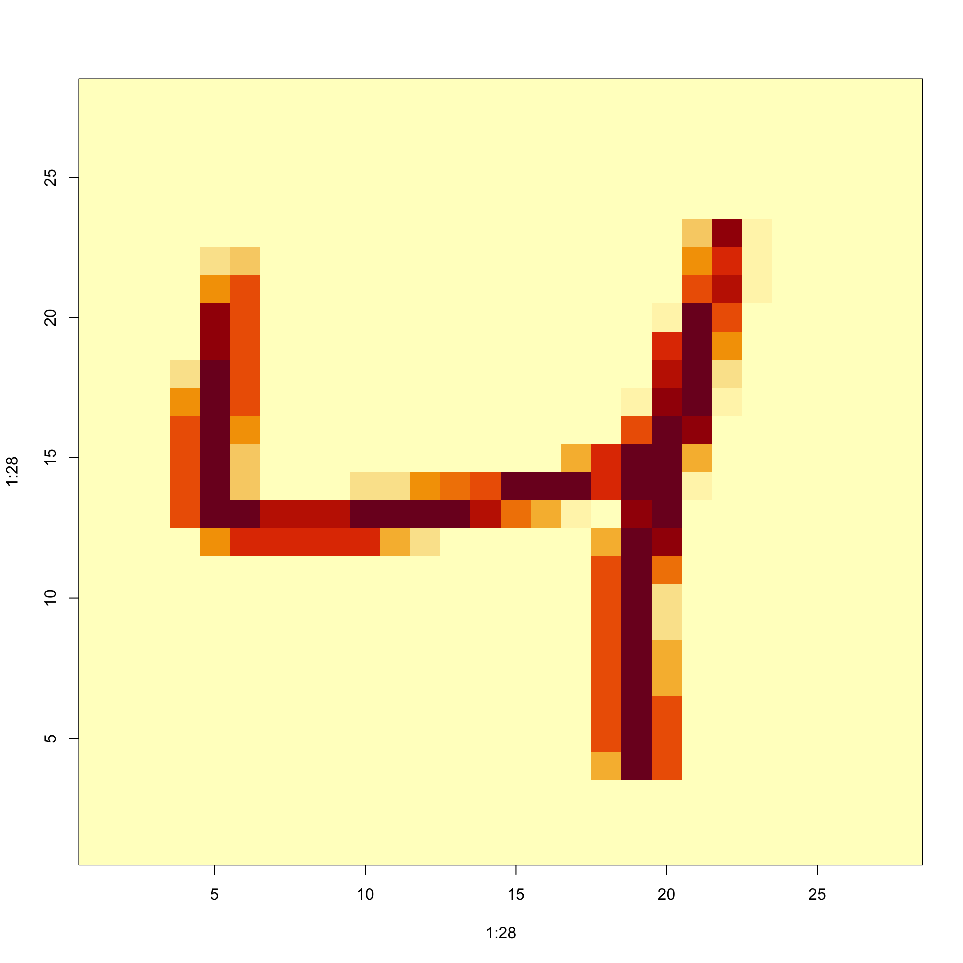
Visualize the original image
- Let’s try to visualize the third observation.
Visualize the original image
The third row of the matrix
x[3,]contains the 784 pixel intensities.We can assume these were entered in order and convert them back to a \(28 \times 28\) matrix using:
Visualize the original image
- To visualize the data, we can use
imagein the followin way:
Visualize the original image
- To flip it back we can use:
Row and column summaries
A common operation with matrices is to apply the same function to each row or to each column.
For example, we may want to compute row averages and standard deviations.
The
applyfunction lets you do this.The first argument is the matrix, the second is the dimension, 1 for rows, 2 for columns, and the third is the function to be applied.
Row and column summaries
- So, for example, to compute the averages and standard deviations of each row, we write:
- To compute these for the columns, we simply change the 1 to a 2:
Row and column summaries
Because these operations are so common, special functions are available to perform them.
The functions
rowMeanscomputes the average of each row:
- and the matrixStats function
rowSdscomputes the standard deviations for each row:
Row and column summaries
The functions
colMeansandcolSdsprovide the version for columns.For more fast implementations consider the functions available in matrixStats.
Do some digits require more ink to write than others?
For the second task, related to total pixel darkness, we want to see the average use of ink plotted against digit.
We have already computed this average and can generate a boxplot to answer the question:
Do some digits require more ink to write than others?

Conditional filtering
One of the advantages of matrices operations over tidyverse operations is that we can easily select columns based on summaries of the columns.
Note that logical filters can be used to subset matrices in a similar way in which they can be used to subset vectors.
Conditional filtering
- Here is a simple example subsetting columns with logicals:
     [,1] [,2] [,3]
[1,]    4    7   13
[2,]    5    8   14
[3,] 6 9 15- This implies that we can select rows with conditional expression.
Conditional filtering
- In the following example we remove all observations containing at least one
NA:
- This being a common operation, we have a matrixStats function to do it faster:
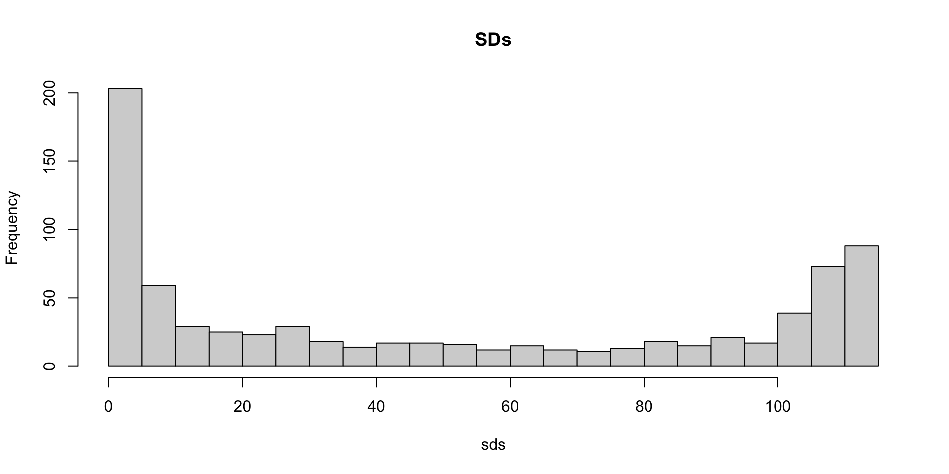
Are some pixels uninformative?
We can use these ideas to remove columns associated with pixels that don’t change much and thus do not inform digit classification.
We will quantify the variation of each pixel with its standard deviation across all entries.
Are some pixels uninformative?
- Since each column represents a pixel, we use the
colSdsfunction from the matrixStats package:
Are some pixels uninformative?
- A quick look at the distribution of these values shows that some pixels have very low entry to entry variability:
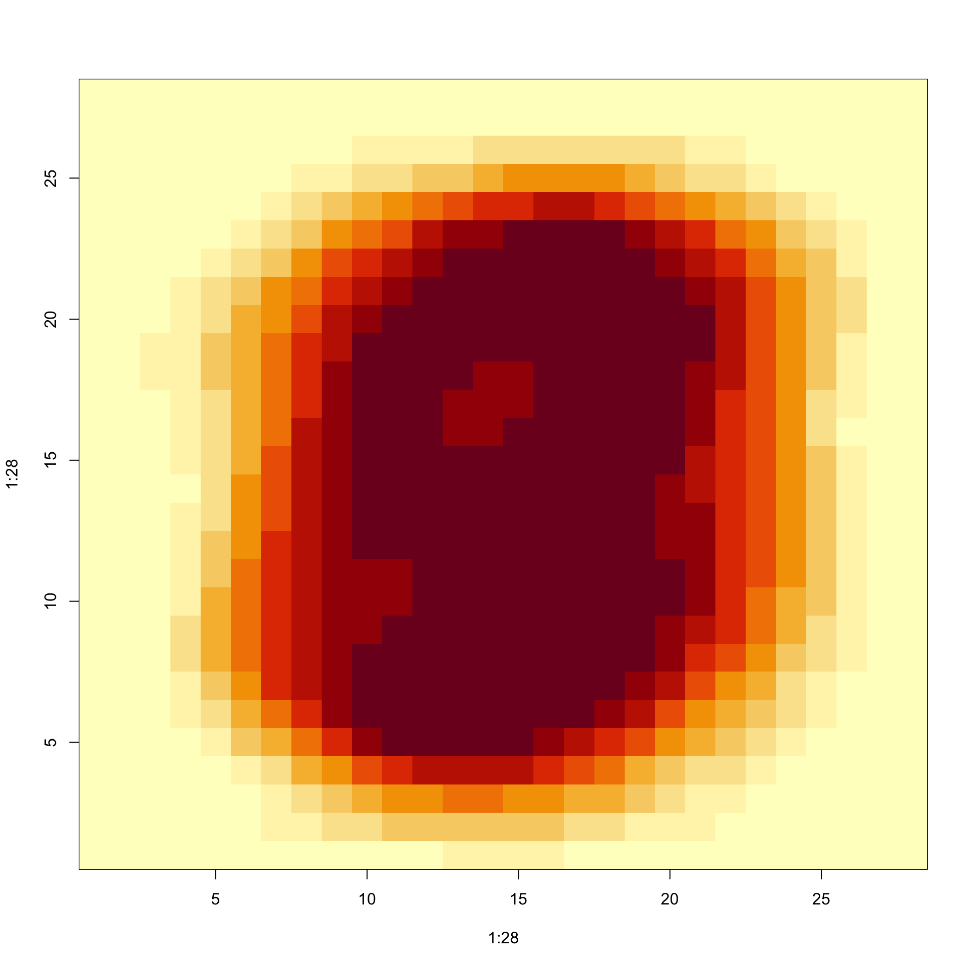
Are some pixels uninformative?
- Here is the variance plotted by location:
Are some pixels uninformative?
We could remove features that have no variation since these can’t help us predict.
So if we wanted to remove uninformative predictors from our matrix, we could write this one line of code:
- Only the columns for which the standard deviation is above 60 are kept, which removes over half the predictors.
Indexing with matrices
An operation that facilitates efficient coding is that we can change entries of a matrix based on conditionals applied to that same matrix.
Here is a simple example:
Indexing with matrices
- A useful application is that we can change all the
NAentries of a matrix to something else:
Can we remove smudges?
- A histogram of all our predictor data:
Can we remove smudges?
The plot shows a clear dichotomy which is explained as parts of the image with ink and parts without.
If we think that values below, say, 50 are smudges, we can quickly make them zero using:
Binarizing the data
The previous histogram seems to suggest that this data is mostly binary.
A pixel either has ink or does not.
Binarizing the data
- Applying what we have learned, we can binarize the data using just matrix operations:
Binarizing the data
- We can also convert to a matrix of logicals and then coerce to numbers like this:
Vectorization for matrices
- In R, if we subtract a vector from a matrix, the first element of the vector is subtracted from the first row, the second element from the second row, and so on.
Vectorization for matrices
- Using mathematical notation, we would write it as follows:
\[ \begin{bmatrix} X_{1,1}&\dots & X_{1,p} \\ X_{2,1}&\dots & X_{2,p} \\ & \vdots & \\ X_{n,1}&\dots & X_{n,p} \end{bmatrix} - \begin{bmatrix} a_1\\\ a_2\\\ \vdots\\\ a_n \end{bmatrix} = \begin{bmatrix} X_{1,1}-a_1&\dots & X_{1,p} -a_1\\ X_{2,1}-a_2&\dots & X_{2,p} -a_2\\ & \vdots & \\ X_{n,1}-a_n&\dots & X_{n,p} -a_n \end{bmatrix} \]
Vectorization for matrices
The same holds true for other arithmetic operations.
The function
sweepfacilitates this type of operation.It works similarly to
apply.It takes each entry of a vector and applies an arithmetic operation to the corresponding row.
Vectorization for matrices
Subtraction is the default arithmetic operation.
So, for example, to center each row around the average, we can use:
Standardize the digits
- The way R vectorizes arithmetic operations implies that we can scale each row of a matrix as follows:
Standardize the digits
Yet this approach does not work for columns.
For columns, we can
sweep:
Standardize the digits
- To divide by the standard deviation, we change the default arithmetic operation to division as follows:
Componentwise multiplication
In R, if you add, subtract, multiple or divide two matrices, the operation is done elementwise.
For example, if two matrices are stored in
xandy, then:
does not result in matrix multiplication.
Instead, the entry in row \(i\) and column \(j\) of this product is the product of the entry in row \(i\) and column \(j\) of
xandy, respectively.