Tidying data

2024-09-25

Tidying data

  • We will a wide format dataset as an example:
library(tidyverse) 
library(dslabs)
path <- system.file("extdata", package = "dslabs")
filename <- file.path(path, "fertility-two-countries-example.csv")
wide_data <- read_csv(filename)
select(wide_data, 1:10)
# A tibble: 2 × 10
  country     `1960` `1961` `1962` `1963` `1964` `1965` `1966` `1967` `1968`
  <chr>        <dbl>  <dbl>  <dbl>  <dbl>  <dbl>  <dbl>  <dbl>  <dbl>  <dbl>
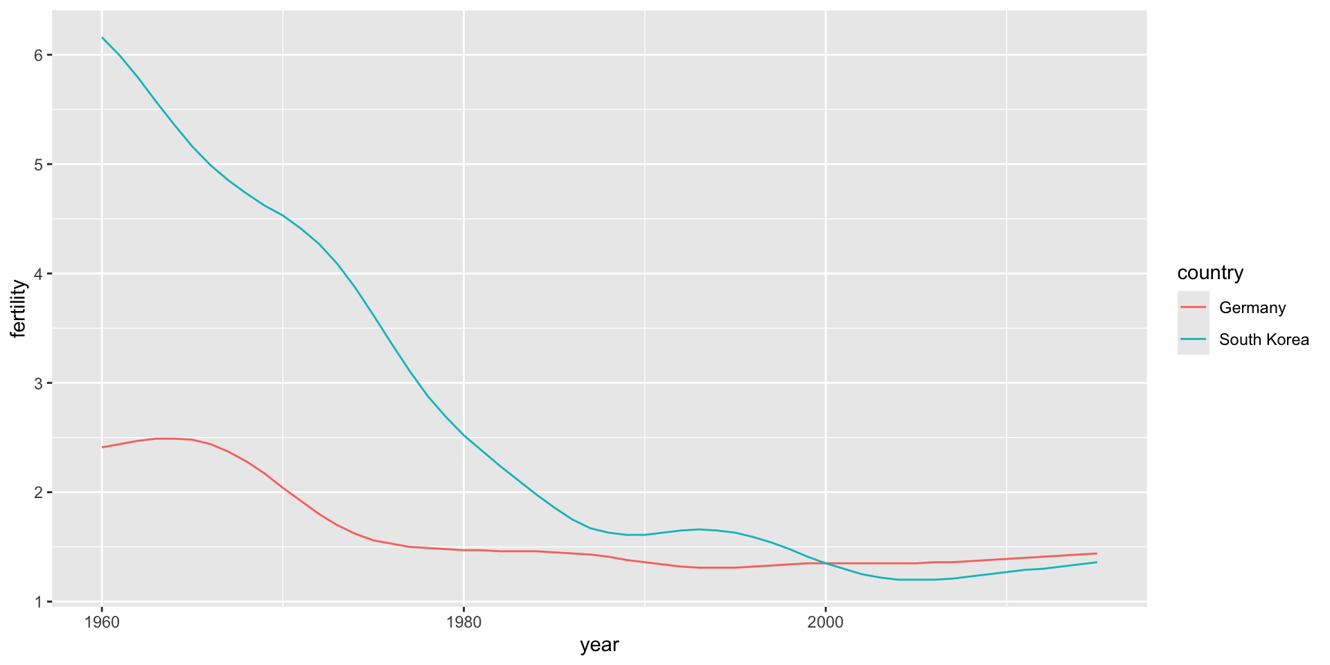
1 Germany       2.41   2.44   2.47   2.49   2.49   2.48   2.44   2.37   2.28
2 South Korea   6.16   5.99   5.79   5.57   5.36   5.16   4.99   4.85   4.73

pivot_longer

  • One of the most used functions in tidyr is pivot_longer.

  • The first argument is a data frame, the one that will be converted.

  • We want to reshape rows represents a fertility observation.

  • We need three columns to store the year, country, and the observed value.

pivot_longer

  • In its current form, data from different years are in different columns with the year values stored in the column names.

  • The names_to and values_to argument tell pivot_longer the column names we want to assign to the columns containing the current column names and observations, respectively.

  • The default names are name and value, in our case a better choice is year and fertility.

pivot_longer

  • Through cols, the second argument, we specify the columns containing observed values; these are the columns that will be pivoted.

  • The default is to pivot all columns so, in most cases, we have to specify the columns. In our example we want columns 1960, 1961 up to 2015.

pivot_longer

The code to pivot the fertility data therefore looks like this:

new_tidy_data <- wide_data |>
  pivot_longer(`1960`:`2015`, names_to = "year", values_to = "fertility")
head(new_tidy_data)
# A tibble: 6 × 3
  country year  fertility
  <chr>   <chr>     <dbl>
1 Germany 1960       2.41
2 Germany 1961       2.44
3 Germany 1962       2.47
4 Germany 1963       2.49
5 Germany 1964       2.49
6 Germany 1965       2.48
  • Data have been converted to tidy format with columns year and fertility.

pivot_longer

  • A quicker way to write this code is to specify which column will not include in the pivot:
new_tidy_data <- wide_data |>
  pivot_longer(-country, names_to = "year", values_to = "fertility")

pivot_longer

  • Now that the data is tidy, we can use it with other tidyverse functions, such ggplot2:
new_tidy_data |> 
  mutate(year = as.numeric(year)) |>
  ggplot(aes(year, fertility, color = country)) + 
  geom_line()

pivot_wider

  • It is sometimes useful for data wrangling purposes to convert tidy data into wide data.

  • We often use this as an intermediate step in tidying up data.

  • The pivot_wider function is basically the inverse of pivot_longer.

pivot_wider

  • The first argument is for the data, but since we are using the pipe, we don’t show it.

  • The names_from argument tells pivot_wider which variable will be used as the column names.

  • The values_from argument specifies which variable to use to fill out the cells.

pivot_wider

Here is some example code

new_wide_data <- new_tidy_data |> 
  pivot_wider(names_from = year, values_from = fertility)
select(new_wide_data, country, `1960`:`1967`)
# A tibble: 2 × 9
  country     `1960` `1961` `1962` `1963` `1964` `1965` `1966` `1967`
  <chr>        <dbl>  <dbl>  <dbl>  <dbl>  <dbl>  <dbl>  <dbl>  <dbl>
1 Germany       2.41   2.44   2.47   2.49   2.49   2.48   2.44   2.37
2 South Korea   6.16   5.99   5.79   5.57   5.36   5.16   4.99   4.85

Similar to pivot_wider, names_from and values_from default to name and value.

Example

We now demonstrate with a more complex example in which we have to use both pivot_longer and pivot_wider to tidy the data.

path <- system.file("extdata", package = "dslabs")

filename <- "life-expectancy-and-fertility-two-countries-example.csv"
filename <-  file.path(path, filename)

raw_dat <- read_csv(filename)
select(raw_dat, 1:5)
# A tibble: 2 × 5
  country     `1960_fertility` `1960_life_expectancy` `1961_fertility`
  <chr>                  <dbl>                  <dbl>            <dbl>
1 Germany                 2.41                   69.3             2.44
2 South Korea             6.16                   53.0             5.99
# ℹ 1 more variable: `1961_life_expectancy` <dbl>

Example

  • Note that the data is in wide format.

  • Also that this table includes values for two variables, fertility and life expectancy, with the column name encoding which column represents which variable.

  • Encoding information in the column names is not recommended but, unfortunately, it is quite common.

Example

  • We start with the pivot_longer function, but we should no longer use the column name year for the new column since it also contains the variable type.

  • We will call it name, the default, for now:

raw_dat |> pivot_longer(-country) |> head()
# A tibble: 6 × 3
  country name                 value
  <chr>   <chr>                <dbl>
1 Germany 1960_fertility        2.41
2 Germany 1960_life_expectancy 69.3 
3 Germany 1961_fertility        2.44
4 Germany 1961_life_expectancy 69.8 
5 Germany 1962_fertility        2.47
6 Germany 1962_life_expectancy 70.0 

Example

  • The result is not exactly what we refer to as tidy since each observation is associated with two, not one, rows.

  • We want to have the values from the two variables, fertility and life expectancy, in two separate columns.

  • The first challenge to achieve this is to separate the name column into the year and the variable type.

Example

  • Encoding multiple variables in a column name is such a common problem that the tidyr package includes function to separate these columns into two or more:
raw_dat |> 
  pivot_longer(-country) |> 
  separate_wider_delim(name, delim = "_",  names = c("year", "name"), 
                       too_many = "merge") |>
  head()
# A tibble: 6 × 4
  country year  name            value
  <chr>   <chr> <chr>           <dbl>
1 Germany 1960  fertility        2.41
2 Germany 1960  life_expectancy 69.3 
3 Germany 1961  fertility        2.44
4 Germany 1961  life_expectancy 69.8 
5 Germany 1962  fertility        2.47
6 Germany 1962  life_expectancy 70.0 

Example

  • But we are not done yet.

  • We need to create a column for each variable and change year to a number.

  • As we learned, the pivot_wider function can do this.

Example

dat <- raw_dat |> 
  pivot_longer(-country) |> 
  separate_wider_delim(name, delim = "_", 
                       names = c("year", "name"), 
                       too_many = "merge") |>
  pivot_wider() |>
  mutate(year = as.integer(year))
head(dat)
# A tibble: 6 × 4
  country  year fertility life_expectancy
  <chr>   <int>     <dbl>           <dbl>
1 Germany  1960      2.41            69.3
2 Germany  1961      2.44            69.8
3 Germany  1962      2.47            70.0
4 Germany  1963      2.49            70.1
5 Germany  1964      2.49            70.7
6 Germany  1965      2.48            70.6

Example

The data is now is now in tidy form and we can use with other packages:

p1 <- dat |> ggplot(aes(year, fertility, color = country)) + geom_line(show.legend = FALSE)
p2 <- dat |> ggplot(aes(year, life_expectancy, color = country)) + geom_line()
gridExtra::grid.arrange(p1, p2, ncol = 2, widths = c(3,4))