R Basics

2024-09-16

Packages

Use install.packages to install the dslabs package.
Tryout the following functions: sessionInfo, installed.packages

Prebuilt functions

Much of what we do in R is based on prebuilt functions.
Many are included in automatically loaded packages: stats, graphics, grDevices, utils, datasets, methods.
This subset of the R universe is refereed to as R base.
Very popular packages not included in R base: ggplot2, dplyr, tidyr, and data.table.

Important

For problem set 2 you can only use R base.

Prebuilt functions

Example of prebuilt functions that we will use today: ls, rm, library, search, factor, list, exists, str, typeof, and class.
You can see the raw code for a function by typing it without the parenthesis: type ls on your console to see an example.

Help system

In R you can use ? or help to learn more about functions.
You can learn about function using

help("ls")

?ls

The workspace

Define a variable.

a <- 2

Use ls to see if it’s there. Also take a look at the Environment tab in RStudio.

ls()

[1] "a"

Use rm to remove the variable you defined.

rm(a)

Variable name convention

A nice convention to follow is to use meaningful words that describe what is stored, use only lower case, and use underscores as a substitute for spaces.
For more we recommend this guide.

Data types

The main data types in R are:

One dimensional vectors: numeric, integer, logical, complex, characters.
Factors
Lists: this includes data frames.
Arrays: Matrices are the most widely used.
Date and time
tibble
S4 objects

Data types

Many errors in R come from confusing data types.
str stands for structure, gives us information about an object.
typeof gives you the basic data type of the object. It reveals the lower-level, more fundamental type of an object in R’s memory.
class This function returns the class attribute of an object. The class of an object is essentially type_of at a higher, often user-facing level.

Data types

Let’s see some example:

library(dslabs)
typeof(murders)

[1] "list"

class(murders)

[1] "data.frame"

str(murders)

'data.frame':   51 obs. of  5 variables:
 $ state     : chr  "Alabama" "Alaska" "Arizona" "Arkansas" ...
 $ abb       : chr  "AL" "AK" "AZ" "AR" ...
 $ region    : Factor w/ 4 levels "Northeast","South",..: 2 4 4 2 4 4 1 2 2 2 ...
 $ population: num  4779736 710231 6392017 2915918 37253956 ...
 $ total     : num  135 19 232 93 1257 ...

Data frames

Date frames are the most common class used in data analysis. It is like a spreadsheet.
Usually, rows represents observations and columns variables.
Each variable can be a different data type.
You can see part of the content like this

head(murders)

       state abb region population total
1    Alabama  AL  South    4779736   135
2     Alaska  AK   West     710231    19
3    Arizona  AZ   West    6392017   232
4   Arkansas  AR  South    2915918    93
5 California  CA   West   37253956  1257
6   Colorado  CO   West    5029196    65

Data frames

and all of the content like this:

View(murders)

Type the above in RStudio.

Data frames

A very common operation is adding columns like this:

murders$pop_rank <- rank(murders$population)
head(murders)

       state abb region population total pop_rank
1    Alabama  AL  South    4779736   135       29
2     Alaska  AK   West     710231    19        5
3    Arizona  AZ   West    6392017   232       36
4   Arkansas  AR  South    2915918    93       20
5 California  CA   West   37253956  1257       51
6   Colorado  CO   West    5029196    65       30

Data frames

Note that we used $.
This is called the accessor because it lets us access columns.

murders$population

 [1]  4779736   710231  6392017  2915918 37253956  5029196  3574097   897934
 [9]   601723 19687653  9920000  1360301  1567582 12830632  6483802  3046355
[17]  2853118  4339367  4533372  1328361  5773552  6547629  9883640  5303925
[25]  2967297  5988927   989415  1826341  2700551  1316470  8791894  2059179
[33] 19378102  9535483   672591 11536504  3751351  3831074 12702379  1052567
[41]  4625364   814180  6346105 25145561  2763885   625741  8001024  6724540
[49]  1852994  5686986   563626

More generally: used to access components of a list.

Data frames

One way R confuses beginners is by having multiple ways of doing the same thing.
For example you can access the 4th column in the following five different ways:

murders$population
murders[, "population"]
murders[["population"]]
murders[, 4]
murders[[4]]

In general, we recommend using the name rather than the number as it is less likely to change.

with

with let’s us use the column names as objects.
This is convenient to avoid typing the data frame name over and over:

rate <- with(murders, total/population)

with

Note you can write entire code chunks by enclosing it in curly brackets:

with(murders, {
   rate <- total/population
   rate <- round(rate*10^5)
   print(rate[1:5])
})

[1] 3 3 4 3 3

Vectors

The columns of data frames are an example of one dimensional (atomic) vectors.

length(murders$population)

[1] 51

Vectors

Often we have to create vectors.
The concatenate function c is the most basic way used to create vectors:

x <- c("b", "s", "t", " ", "2", "6", "0")

Sequences

Sequences are a the common example of vectors we generate.

seq(1, 10)

 [1]  1  2  3  4  5  6  7  8  9 10

seq(1, 9, 2)

[1] 1 3 5 7 9

When increasing by 1 you can use :

1:10

 [1]  1  2  3  4  5  6  7  8  9 10

Sequences

A useful function to quickly generate the sequence 1:length(x) is seq_along:

x <- c("b", "s", "t", " ", "2", "6", "0")
seq_along(x)

[1] 1 2 3 4 5 6 7

A reason to use this is to loop through entries:

for (i in seq_along(x)) {
  cat(toupper(x[i]))
}

BST 260

Factors

One key distinction between data types you need to understad is the difference between factors and characters.
The murder dataset has examples of both.

class(murders$state)

[1] "character"

class(murders$region)

[1] "factor"

Why do you think this is?

Factors

Factors store levels and the label of each level.
This is useful for categorical data.

x <- murders$region
levels(x)

[1] "Northeast"     "South"         "North Central" "West"

Categories based on strata

In data analysis we often have to stratify continuous variables into categories.
The function cut helps us do this:

age <- c(5, 93, 18, 102, 14, 22, 45, 65, 67, 25, 30, 16, 21)
cut(age, c(0, 11, 27, 43, 59, 78, 96, Inf))

 [1] (0,11]   (78,96]  (11,27]  (96,Inf] (11,27]  (11,27]  (43,59]  (59,78] 
 [9] (59,78]  (11,27]  (27,43]  (11,27]  (11,27] 
Levels: (0,11] (11,27] (27,43] (43,59] (59,78] (78,96] (96,Inf]

Categories based on strata

We can assign it more meaningful level names:

age <- c(5, 93, 18, 102, 14, 22, 45, 65, 67, 25, 30, 16, 21)
cut(age, c(0, 11, 27, 43, 59, 78, 96, Inf), 
    labels = c("Alpha", "Zoomer", "Millennial", "X", "Boomer", "Silent", "Greatest"))

 [1] Alpha      Silent     Zoomer     Greatest   Zoomer     Zoomer    
 [7] X          Boomer     Boomer     Zoomer     Millennial Zoomer    
[13] Zoomer    
Levels: Alpha Zoomer Millennial X Boomer Silent Greatest

Changing levels

This is often needed for ordinal data because R defaults to alphabetical order:

gen <- factor(c("Alpha", "Zoomer", "Millennial"))
levels(gen)

[1] "Alpha"      "Millennial" "Zoomer"

You can change this with the levels argument:

gen <- factor(gen, levels = c("Alpha", "Zoomer", "Millennial", "X", "Boomer", "Silent", "Greatest"))
levels(gen)

[1] "Alpha"      "Zoomer"     "Millennial" "X"          "Boomer"    
[6] "Silent"     "Greatest"

Changing levels

A common reason we need to change levels is to assure R is aware which is the reference strata.
This is important for linear models because the first level is assumed to be the reference.

x <- factor(c("no drug", "drug 1", "drug 2"))
levels(x)

[1] "drug 1"  "drug 2"  "no drug"

x <- relevel(x, ref = "no drug")
levels(x)

[1] "no drug" "drug 1"  "drug 2"

Changing levels

We often want to order strata based on a summary statistic.
This is common in data visualization.
We can use reorder for this:

x <- reorder(murders$region, murders$population, sum)

Factors

Another reason we used factors is because they more efficient:

x <- sample(murders$state[c(5,33,44)], 10^7, replace = TRUE)
y <- factor(x)
object.size(x)

80000232 bytes

object.size(y)

40000648 bytes

An integer is easier to store than a character string.

Factors

Exercise: How can we make this go much faster?

system.time({levels(y) <- tolower(levels(y))})

   user  system elapsed 
  0.018   0.000   0.019

Factors can be confusing

Try to make sense of this:

x <- factor(c("3","2","1"), levels = c("3","2","1"))
as.numeric(x)

[1] 1 2 3

x[1]

[1] 3
Levels: 3 2 1

levels(x[1])

[1] "3" "2" "1"

table(x[1])


3 2 1 
1 0 0

Factors can be confusing

Avoid keeping extra levels with droplevels:

z <- x[1]
z <- droplevels(z)

But note what happens if we change to another level:

z[1] <- "1"
z

[1] <NA>
Levels: 3

NAs

NA stands for not available.
Data analysts have to deal with NAs often.

NAs

dslabs includes an example dataset with NAs

library(dslabs)
na_example[1:20]

 [1]  2  1  3  2  1  3  1  4  3  2  2 NA  2  2  1  4 NA  1  1  2

The is.na function is key for dealing with NAs

is.na(na_example[1])

[1] FALSE

is.na(na_example[17])

[1] TRUE

is.na(NA)

[1] TRUE

is.na("NA")

[1] FALSE

NAs

Technically NA is a logical

class(NA)

[1] "logical"

When used with ands and ors, NAs behaves like FALSE

TRUE & NA

[1] NA

TRUE | NA

[1] TRUE

But NA is not FALSE. Try this:

if (NA) print(1) else print(0)

NaNs

A related constant is NaN.
Unlike NA, which is a logical, NaN is a number.
It is a numeric that is Not a Number.
Here are some examples:

0/0

[1] NaN

class(0/0)

[1] "numeric"

sqrt(-1)

[1] NaN

log(-1)

[1] NaN

Coercing

When you do something inconsistent with data types, R tries to figure out what you mean and change it accordingly.
We call this coercing.
R does not return an error and in some cases does not return a warning either.
This can cause confusion and unnoticed errors.
So it’s important to understand how and when it happens.

Coercing

Here are some examples:

typeof(1L)

[1] "integer"

typeof(1)

[1] "double"

typeof(1 + 1L)

[1] "double"

c("a", 1, 2)

[1] "a" "1" "2"

TRUE + FALSE

[1] 1

factor("a") == "a"

[1] TRUE

identical(factor("a"), "a")

[1] FALSE

Coercing

When R can’t figure out how to coerce, rather an error it returns an NA:

as.numeric("a")

[1] NA

Note that including NAs in arithmetical operations usually returns an NA.

1 + 2 + NA

[1] NA

Coercing

You want to avoid automatic coercion and instead explicitly do it.
Most coercion functions start with as.
Here is an example.

x <- factor(c("a","b","b","c"))
as.character(x)

[1] "a" "b" "b" "c"

as.numeric(x)

[1] 1 2 2 3

Coercing

More examples:

x <- c("12323", "12,323")
as.numeric(x)

[1] 12323    NA

library(readr)
parse_guess(x)

[1] 12323 12323

Lists

Data frames are a type of list.
Lists permit components of different types and, unlike data frames, different lengths:

x <- list(name = "John", id = 112, grades = c(95, 87, 92))

The JSON format is best represented as list in R.

Lists

You can access components in different ways:

x$name

[1] "John"

x[[1]]

[1] "John"

x[["name"]]

[1] "John"

Matrics

Matrices are another widely used data type.
They are similar to data frames except all entries need to be of the same type.
We will learn more about matrices in the High Dimensional data Analysis part of the class.

Functions

You can define your own function. The form is like this:

f <- function(x, y, z = 0){
  ### do calculations with x, y, z to compute object
  ## return(object)
}

Functions

Here is an example of a function that sums $1,2,\dots,n$

s <- function(n){
   return(sum(1:n))
}

Lexical scope

Study what happens here:

f <- function(x){
  cat("y is", y,"\n")
  y <- x
  cat("y is", y,"\n")
  return(y)
}
y <- 2
f(3)

y is 2 
y is 3

[1] 3

y <- f(3)

y is 2 
y is 3

[1] 3

Namespaces

Look at how this function changes by typing the following:

filter
library(dplyr)
filter

Namespaces

Note what R searches the Global Environment first.
Use search to see other environments R searches.
Note many prebuilt functions are in stats.

Namespaces

You can explicitly say which filter you want using namespaces:

stats::filter
dplyr::filter

Namespaces

Restart yoru R Consuole and study this example:

library(dslabs)
exists("murders")

[1] TRUE

murders <- murders
murders2 <- murders
rm(murders)
exists("murders")

[1] TRUE

detach("package:dslabs")
exists("murders")

[1] FALSE

exists("murders2")

[1] TRUE

Object Oriented Programming

R uses object oriented programming (OOP).
It uses two approaches referred to as S3 and S4, respectively.
S3, the original approach, is more common.
The S4 approach is more similar to the conventions used by modern OOP languages.

plot(co2)

plot(as.numeric(co2))

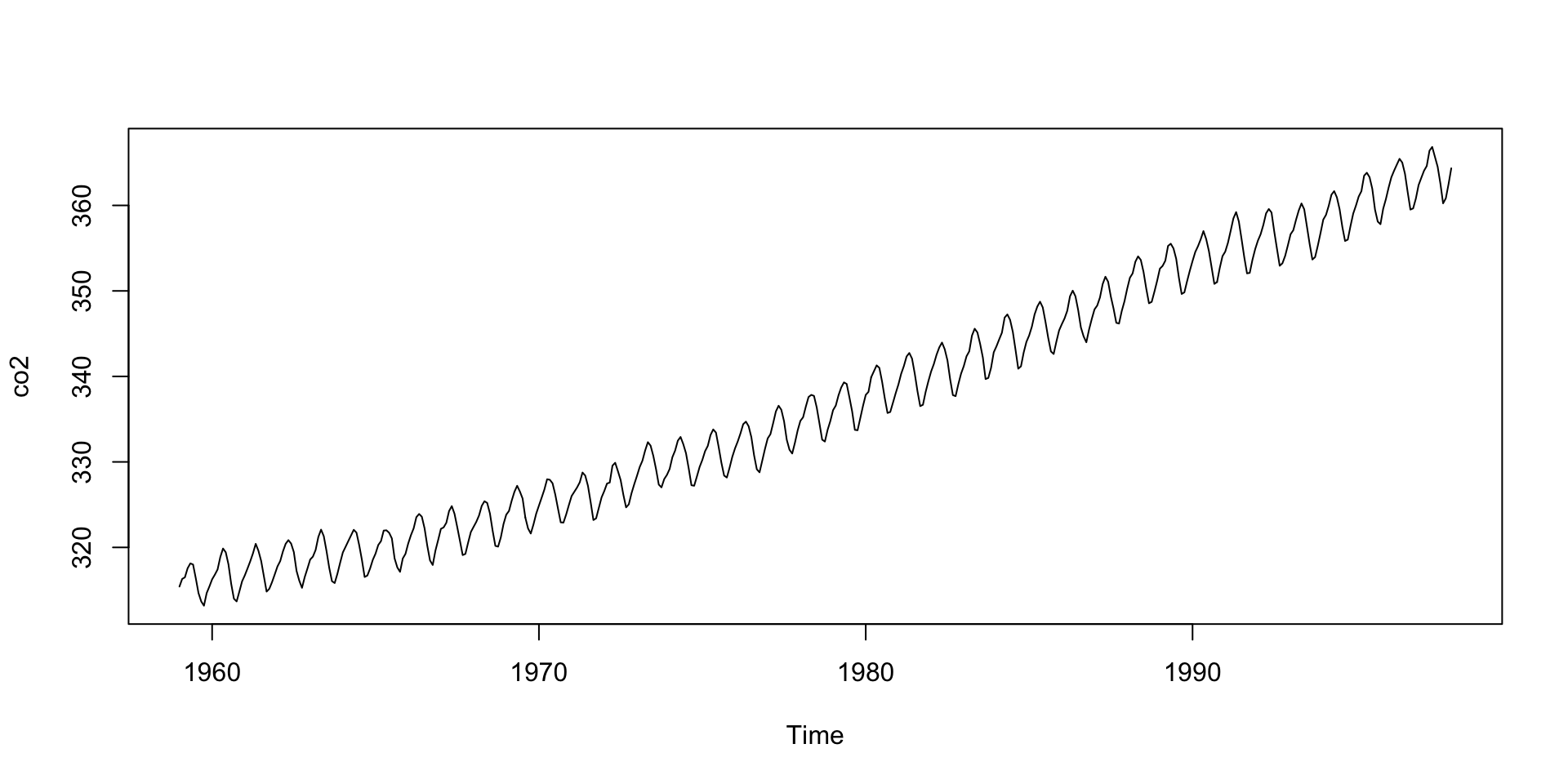
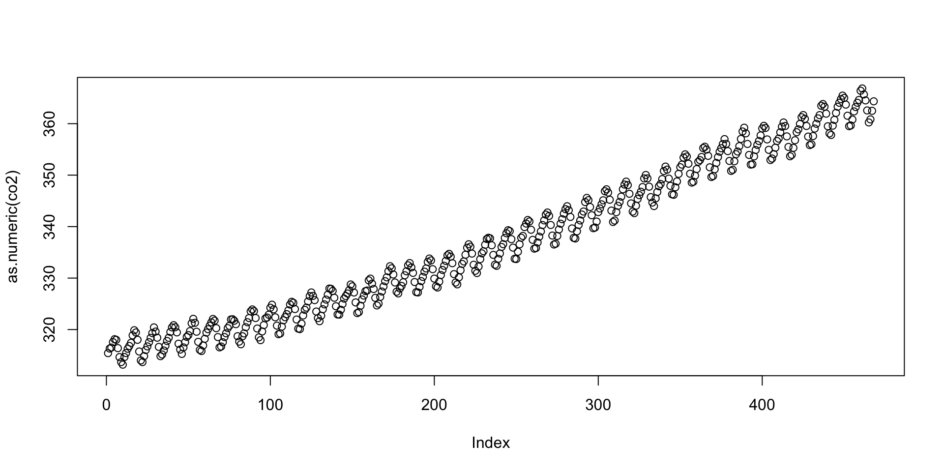
Object Oriented Programming

Note co2 is not numeric:

class(co2)

[1] "ts"

The plots are different because plot behaves different with different classes.

Object Oriented Programming

The first plot actually calls the function

plot.ts

Notice all the plot functions that start with plot by typing plot. and then tab.
The function plot will call different functions depending on the class of the arguments.

Plots

Soon we will learn how to use the ggplot2 package to make plots.
R base does have functions for plotting though
Some you should know about are:
- plot - mainly for making scatterplots.
- lines - add lines/curves to an existing plot.
- hist - to make a histogram.
- boxplot - makes boxplots.
- image - uses color to represent entries in a matrix.

Plots

Although, in general, we recommend using ggplot2, R base plots are often better for quick exploratory plots.
For example, to make a histogram of values in x simply type:

hist(x)

To make a scatter plot of y versus x and then interpolate we type:

plot(x,y)
lines(x,y)